CHAPTER 24
Antenna Tuners (ATUs)
The primary task of an impedance-matching or antenna tuning unit (ATU) located at the transmitter end of the transmission line is to present the transmitter output stage with an apparent antenna feedpoint impedance (after transformation through an arbitrary-length transmission line) equal to the output impedance of the transmitter. This results in maximum power transfer from the power amplifier stage of the transmitter to the feedline and antenna. So located, a properly designed ATU provides the station owner with multiple benefits:
• It minimizes the standing wave ratio (SWR) that the transmitter or power amplifier—whether vacuum tube or solid-state—sees. RF power amplifiers are not tolerant of high SWR; when operating into a mismatched load, expensive tubes, transistor(s), and other components can be destroyed instantly.
• It minimizes the occurrence of reduced output power triggered by power amplifier “fold-back” protection circuitry when a high VSWR is sensed.
• It facilitates operation of the transmitter final amplifier stage at maximum efficiency.
• It provides additional attenuation of out- of- band emissions, including harmonics generated in, or amplified by, the amplifier.
• If left in the line to the receiver during “key up” periods, it helps protect the receiver from overload caused by strong out- of- band signals.
If, on the other hand, the ATU is located at the antenna end of the transmission line, it not only accomplishes all those benefits listed here but it also transforms the feedpoint impedance of the antenna to the system impedance or principal station transmission line impedance—totally eliminating the reactive part of the feedpoint impedance and presenting the transmission line with an RRAD that is identical to Z0. Thus, an ATU located at the antenna provides the user with the following additional benefits:
• It minimizes the occurrence and amplitude of high-voltage standing waves along the line that can destroy the transmission line and any associated switches, relays, or other components when high power is employed.
• It minimizes additional, or mismatch, signal loss on long transmission lines relative to the loss that is present with line SWRs greater than 1.0:1.
• It can include additional protection for station electronics (receivers, transmitters, accessories, etc.) from lightning-induced events, serving as a first line of defense in preventing voltage or current surges from entering the radio room.
As the second set of bullets makes clear, it is generally preferable to locate the ATU at the antenna. However, at low frequencies, low power levels, and/or for relatively short distances between the transmitter output and the antenna, an ATU at the transmitter can provide acceptable results (except with respect to keeping lightning out of the radio shack). Today most commercially available transceivers sport an internal ATU—either standard or as an option. When operated “barefoot” (i.e., with no amplifier) and with short feedlines (such as mobile or portable installations) on HF, this configuration is compact and provides nearly as efficient power transfer to the antenna as a separate box located at the antenna would.
In many stations, however, the approach is to incorporate matching devices at both ends of the system transmission line—that is, to locate fixed-tuned impedance-matching networks at the antenna feedpoint to get the SWR on the system transmission line down to a manageable level and a tunable ATU back at the transmitter and receiver end of the main transmission line to complete the task of presenting the transmitter with a matched load, especially when the operating frequency is apt to be varied by a modest amount— typically no more than a few percent. Often, the impedance-matching network at the antenna is a simple balun or a distributed network, such as the transmission line transformers described in the second half of Chap. 4.
Occasionally fully tunable ATUs are located at or near the antenna end of the system transmission line. In that case, they are often capable of being tuned remotely, or the intended operating range is over such a small percentage bandwidth that adjustment of the ATU is required infrequently or never. An example of such a configuration is found in Fig. 8.2; open-wire line (which is the best choice when the possibility of high SWR on the line exists) connects the center of a multiband dipole to a tunable ATU directly beneath it. The ATU is adjusted to provide minimum SWR on the coaxial transmission line that comes from the station equipment. It may also incorporate RF chokes to drain static buildup from the antenna and OWL, or remotely actuated mechanical contactors to directly ground the OWL and dipole when they’re not in use. An even more compelling case for a remote ATU is the bobtail curtain of Chap. 10. Since the feedpoint for this array is at a high-impedance point, the SWR on any common coaxial cable back to the transmitter would put the cable at risk of destruction when substantial power levels are used. Any attempt to run open-wire line over that distance could materially degrade the antenna pattern. Locating a tunable ATU at the base of the antenna, as shown in Fig. 10.11, is by far the best possible approach.
ATU Circuit Configurations
While it is tempting to treat the ATU as a black box, in truth there are many different kinds of impedance-matching circuit configurations, each with its own list of advantages and disadvantages. At any given operating frequency, the antenna feedpoint impedance, ZANT, can be represented as a resistive part, RANT, in series with a reactive part, XANT:
![]()
where XANT can be either positive or negative. If we could count on RANT always equaling the system transmission line impedance, Z0, we could use a single variable capacitor in series to tune out a positive XANT and a single variable inductor in series to tune out a negative XANT. Unfortunately, as the operating frequency changes, not only does XANT vary—often between positive and negative values—but RANT does so, as well. As explained in Chap. 3, neither RANT nor XANT corresponds to a specific resistor, capacitor, or inductor except in the very simplest electronic circuits. The magnitude and frequency dependence of either RANT or XANT—and most likely both—are, in general, complicated functions of many components in a lumped-element circuit and of many geometrical interrelationships in a distributed circuit such as an antenna. Thus, the task of the successful antenna matching unit or ATU is to be flexible enough to present the system transmission line with an apparent antenna feedpoint impedance of ZANT = Z0 = R0 + j0 over a reasonable range of operating frequencies and a practical range of complex antenna impedances. In the process, the ATU should dissipate as little of the transmitter RF power output in internal losses as possible. As you might expect, various network topologies can do this—but with varying degrees of success.
L-Section Network
Judging by the number of times it has appeared in print, the L-section network is one of the most used antenna matching networks in existence, rivaling even the pi network. A typical circuit for one form of L-section network is shown in Fig. 24.1A. Values for L and C can be found that will allow this circuit to match all possible load impedances having R1, the resistive part of the source impedance, less than R2, the resistive part of the load impedance. The circuit can also match some load impedances for the range R1 > R2, depending on the magnitude of X2, the reactive part of the series-representation load impedance. For the special case when both the source and the load impedances are purely resistive, the design equations are:

FIGURE 24.1 (A) L-section network. (B) Reverse L section. (C) Inverted L-section network.
![]()
![]()
where, of course,
![]()
and
![]()
The L-section network of Fig. 24.1B differs from the previous circuit in that the coil and capacitor locations are swapped. As before, values for L and C can be found that will allow this circuit to match all possible load impedances having R1 < R2, and some load impedances for the range R1 > R2, depending on the magnitude of X2. For the special case when both the source and the load impedances are purely resistive, the design equations are:
![]()
![]()
![]()
Figure 24.1C is similar to Fig. 24.1A with the exception that the capacitor is at the input rather than the output of the network. Values for L and C can be found that will allow this topology to match all possible load impedances having R1 > R2, and some load impedances for the range R1 < R2. The equations governing this network are:
![]()
![]()
![]()
Because of the limitations on the range of load impedances it can match when either the source or the load has a reactive component, an L network located at the transmitter end of a feedline should be configurable to accommodate the different topologies shown in Fig. 24.1. Alternatively, an L network located at the antenna feedpoint can be a fixed topology once the nature of the feedpoint impedance of the antenna is known.
Pi Networks
The pi network (or pi-section network) shown in Fig. 24.2 is used to match a high source impedance to a low load impedance. These circuits are typically used in vacuum tube RF power amplifiers that need to match output impedances of a few thousand ohms to much lower system transmission line impedances—typically 50 or 75 Ω. The name of the circuit comes from its resemblance to the Greek letter pi (π). The equations for the pi network are:

![]()
![]()

![]()
![]()
Of course, if R1 < R2, the pi network can be flipped left to right; that is, R1 can become the load and R2 the source. Because the pi network typically has a higher Q than an L-section network, its bandwidth will generally be narrower. If bandwidth is an important issue, a pair of cascaded L sections may be a better solution to a particular matching task.
Split-Capacitor Network
The split-capacitor network shown in Fig. 24.3 is used to transform a source impedance that is less than the load impedance. In addition to matching antennas, this circuit is also used for interstage impedance matching inside communications equipment. The equations for design are:

FIGURE 24.3 Split-capacitor network.
![]()
![]()
![]()
![]()
![]()
Transmatch Circuit
One version of the transmatch is shown in Fig. 24.4. This circuit is basically a combination of the split-capacitor network and an output tuning capacitor (C2). For the HF bands, the capacitors are on the order of 150 pF per section for C1, and 250 pF for C2. The tapped or roller inductor should have a maximum value of 28 μH. A popular use of the transmatch is as a coax- to- coax impedance matcher.

FIGURE 24.4 Split-capacitor transmatch network.
The long-popular E. F. Johnson Matchbox is a fundamentally balanced variant of this circuit, designed primarily for use with balanced feedlines such as open-wire line, twin-lead, et al. In the Matchbox, coupling to the transmitter or receiver is accomplished via an inductive link (an isolated secondary winding on L), thus eliminating the connection of R1 across half of C1. C2 becomes a split capacitor connected across the full length of tapped inductor L, and the junctions of the two halves of C1 and C2 are tied together and grounded to the chassis. Each half of the new C2 is itself split again, and the two sides of the balanced transmission line are connected at the midpoint of the split-capacitor half of C2 on each side of ground. The center conductor of an SO-239 chassis-mounted coaxial receptacle for feeding unbalanced transmission lines is hard-wired to the midpoint of one side of C2.
Perhaps the most common form of transmatch circuit is the tee network shown in Fig. 24.5. Like the reverse L-network of Fig. 24.1B, it is basically a high-pass filter and thus does nothing for transmitter harmonic attenuation.

FIGURE 24.5 Tee-network transmatch.
An alternative network, called the SPC transmatch, is shown in Fig. 24.6. This version of the circuit offers some harmonic attenuation.

FIGURE 24.6 Improved transmatch offers harmonic attenuation.
Lumped-component matching networks (or ATUs) for MF and HF are relatively easy to build, although the cost of inductors and variable capacitors capable of withstanding the voltages and currents associated with transmitter power levels is eye-opening. (Even when purchased used at flea markets or via the Internet, good high-power components are not cheap!) Probably the most important thing to remember when building your own ATU is to leave lots of space between any metallic enclosure and the internal components. Failure to do so can alter the circuit Q and reduce overall efficiency of the unit.
In the early days of radio, very few home-built transmitters or ATUs were shielded. The drive to shield RF-generating circuits gained strength in the 1940s with the spread of television broadcasting and the concomitant potential for interference to the neighbors’ TV reception. Today, all commercially produced transmitters, transceivers, and amplifiers are thoroughly shielded and filtered against the unwanted emission of harmonics and other spurious products of the signal generation and amplification process, so shielding of the ATU may not be seen as an imperative. However, every tuned circuit in the path between transmitter and antenna helps reduce these undesired emissions across some frequency ranges, so total shielding of the ATU circuitry is always the best practice.
Baluns
A balun is a transformer that matches a balanced load (such as a horizontal dipole or Yagi antenna) to an unbalanced resistive source (such as a transmitter output or a coaxial feedline). The baluns discussed in this section are lumped-circuit implementations typically wound on ferrite cores, but baluns can also be formed from sections of transmission line properly interconnected. The latter type is included in the review of distributed matching networks near the end of Chap. 4.
Toroid Impedance-Matching Transformers
The toroidal transformer is capable of providing a broadband match between antenna and transmission line, or between transmission line and transmitter or receiver. The other matching methods (shown thus far) are frequency-sensitive and must be readjusted whenever the operating frequency is changed by even a small percentage. Although this problem is of no great concern to fixed-frequency radio stations, it is of critical importance to stations that operate on a variety of frequencies or widely separated bands of frequencies.
Figure 24.7A shows a trifilar transformer that provides a 1:1 impedance ratio, but it will transform an unbalanced transmission line (e.g., coaxial cable) to a balanced signal required to feed a dipole antenna. Although it provides no impedance transformation, it does tend to balance the feed currents in the two halves of the antenna. This fact makes it possible to obtain a more symmetrical figure eight dipole radiation pattern in the horizontal plane. Many station owners make it standard practice to use a balun at the antenna feedpoint when using coaxial (unbalanced) transmission line, even if the feedpoint impedance is close to the Z0 of the cable.

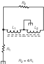
The balun shown in Fig. 24.7B is designed to provide unbalanced to balanced transformation in conjunction with a 4:1 impedance transformation. Thus, a 300-Ω folded dipole feedpoint impedance will be transformed to 75-Ω unbalanced. This type of balun is often included inside ATUs. L1 and L2 have equal turns.
Another multiple-impedance transformer is shown in Fig. 24.7C. In this case, the operator can select impedance transformation ratios of 1.5:1, 4:1, 9:1 or 16:1. A commercial version of this type of transformer, shown in Fig. 24.7D, is manufactured by Palomar Engineers; it’s intended for feeding vertical HF antennas. It will, however, work well in other impedance-transformation applications, too.

FIGURE 24.7C Tapped multiple-impedance BALUN.

FIGURE 24.7D Commercial tapped transformer.
Figures 24.7B and 24.7C are specific examples of what can be accomplished using a toroidal core of the right material and power-handling capability in conjunction with an autoformer winding, where both input and output loads are referenced to a common ground. If ground isolation is important, there is no reason completely separate windings can’t be used, in a configuration analogous to a link-coupled coil.
Ferrite Core Inductors
The word ferrite refers to any of several examples of a class of materials that behave similarly to powdered iron compounds and are used in radio equipment as the cores for inductors and transformers. Although the materials originally employed were of powdered iron (and indeed the name ferrite still implies iron), many modern materials are composed of other compounds. According to literature from Amidon Associates, ferrites with a relative permeability, or μr, of 800 to 5000 are generally of the manganese-zinc type of material, and cores with relative permeabilities of 20 to 800 are of nickel-zinc. The latter are useful in the 0.5- to 100- MHz range.
Toroid Cores
In electronics parlance, a toroid is a doughnut-shaped object made from a ferrite material and used as the form for winding an inductor or transformer. Many different core material formulations are available for the designer to choose from, based on the expected frequency range and power levels of the application.
Unlike just about any other lumped component available to the experimenter, most toroids carry little or no information about themselves on their surface. In general, blindly grabbing an arbitrary toroid from the junk box will lead to a failed project. Toroids must be selected carefully—with the use of a test jig, if necessary.
Charts of product characteristics for toroids are provided by manufacturers such as Amidon and Fair-Rite, and by their distributors, and are best obtained from an Internet search of their sites. In addition, some of these data are also available in The ARRL Handbook for the Radio Amateur. As an example, a T- 50- 2 core is useful from 1 to 30 MHz, has a permeability of 10, is painted red, and has the following dimensions: OD = 0.500 in (1.27 cm), ID = 0.281 in (0.714 cm), and a height (i.e., thickness) of 0.188 in (0.448 cm).
Toroidal Transformers
Windings on a toroid are generally wound simultaneously in a “multifilar” manner. In this approach, multiple wires of equal length are slightly twisted together first, then wrapped around and through the doughnut form as if they were a single winding. The preferred number of wires in parallel is a function of the required step-up or step-down ratio and whether an autotransformer or isolated primary and secondary windings are required. Figure 24.8A is the schematic of a 4:1 balun transformer with separate primary and secondary windings. The dot at the top of each winding indicates the polarity or phase of the winding; for proper operation as an autoformer, all three wires must wrap around the doughnut in the same direction, and the builder must mark the dotted end of all three—conceptually, if not literally—when soldering ends together or bringing them out to connectors. This particular circuit is said to have a trifilar wound core.

FIGURE 24.8 Broadband RF transformer.
Figure 24.8B exposes detail of the trifilar winding. For the sake of clarity, each of the three wires has been drawn with its own simulated insulation “pattern” so that you can more easily see how the winding is formed. Most small construction projects (e.g., Beverage antenna transformers) use #26, #28, or #30 enameled wire to wind coils; consider stocking three colors of each size, so that each winding can be a unique color. For higher-power transmitting antenna baluns, use #16, #14, #12, or #10 wire. Enamel and Teflon are common insulation layers. To help identify wires of these diameters, label their ends with adhesive labels.
Figure 24.9 shows two accepted methods for winding a multifilar coil on a toroidal core. Figure 24.9A is an actual photograph of toroid wound with the method shown pictorially in Fig. 24.8B. Here the wires are laid down parallel to each other, as shown previously. The method of Fig. 24.9B uses twisted wires. Prior to winding the toroid, the three wires are “chucked up” in a drill and twisted together before being wound on the core. With one end of the three wires secured in the drill chuck, anchor their far ends in something that will hold them taut. Some people use a bench vise for this purpose. Run the drill at slow speed and allow the wires to twist together until the desired pitch is achieved. Remember to wear eye protection in case a wire breaks or gets loose from its mooring at the far end.
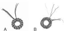
FIGURE 24.9 Winding a toroidal transformer. (A) Parallel wound. (B) Twist wound.
To actually wind the bundle of wires on the toroid, pass the bundle through the doughnut hole until the toroid is about in the middle of the length of wire. Loop the wire over and around the outside surface of the toroid and pass it through the hole again. Repeat this process until the correct number of turns is wound onto the core. Be sure to press the wire against the toroid form, and keep it taut as you wind the coils.
To minimize the chance of a chipped core breaking through the wire insulation, wrap the core with a slightly overlapped layer of fiberglass packing tape before starting to wind. To prevent windings (especially those made with very fine wire) from unwinding, secure the ends of the wires with a tiny dab of rubber cement or RTV silicone sealer.
Mounting Toroid Cores
To mount a properly wound toroidal inductor or transformer, consider these options:
• If the wire is heavy enough, just use the wire connections to the circuit board or terminal strip to support the component—especially if the connections are directly above or below the toroid.
• Smaller, lighter toroids can be laid flat on the circuit board and cemented in place with silicone seal or rubber cement.
• Drill a hole in the wiring board and use a screw and nut to secure the toroid. Do not use metallic hardware for mounting the toroid! Metallic fasteners will alter the inductance of the component and possibly render it unuseable. Use nylon hardware for mounting the toroidal component.
How Many Turns?
Three factors must be taken into consideration when making toroid transformers or inductors: toroid size, core material, and number of turns of wire. Toroid size is a function of power-handling capability and handling/installation convenience. Core material depends on the frequency range of the circuit and the application (balun, common mode choke, etc.).
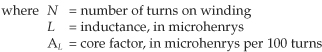
Equation (24.23) provides a rough rule of thumb for the turns count. Based on the availability of a parameter called the AL factor, the number of turns needed to obtain a specified inductance is given by
![]()
Example 24.1 Calculate the number of turns required to make a 5- μH inductor on a T- 50- 6 core. The AL factor for the core is 40.
Solution

Don’t take the value obtained from the equation too seriously, however, because a wide tolerance exists on amateur-grade ferrite cores. Although it isn’t too much of a problem when building baluns and other transformers, it can be a concern when making fixed inductors for a tuned circuit. If the tuned circuit requires considerably more (or less) capacitance than called for in the standard equation, and all of the stray capacitance is properly taken into consideration, the actual AL value of your particular core may be different from the table value.
Ferrite Rods
Another form of ferrite core available on the market is the rod, shown in Fig. 24.10. Often used as a high-current RF choke for the vacuum tube filaments of grounded-grid linear amplifiers, the rod can be pressed into service as a balun, as well. Primary and secondary windings are wound in a bifilar manner over the ferrite rod.

FIGURE 24.10 Ferrite rod inductor construction.
Ferrite rods are also used in receiving antennas—especially when high inductance in a small space is required. Although the amateur use is not extensive, the ferrite rod antenna (or loopstick) is popular in small receivers for MF and below, and in portable radio direction-finding equipment. Some amateurs use sharp nulls of loopstick receiving antennas to null out interfering signals on the crowded HF bands. Of course, you would not want to use a small loopstick rod in a transmitting application.
Ferrite rods are light enough to be suspended from their own wires or to be glued or cemented to a panel or printed circuit board inside the receiver. In place of the simple nylon screws that hold toroids in place, we can use insulating cable clamps to secure the ends of the rod to the board.