CHAPTER 14
Receiving Antennas for High Frequency
Antennas are reciprocal devices. That is, just as transmitter power applied to the feedpoint of an antenna results in a field of a certain strength at a remote point, fields originating remotely can impinge upon that same antenna and create a received signal voltage and power at that same feedpoint.
Under most—but not all—circumstances, the best antenna to use for transmitting is also the best antenna to use for receiving. Sometimes, however, the use of a separate receiving antenna (or antennas) can lead to better reception and an overall improvement in communications reliability. This is especially true for the very low frequency (VLF), low frequency (LF), medium frequency (MF), and lower high-frequency (HF) ranges of the radio spectrum, for any of the following reasons:
• Dimensions and construction costs of effective and efficient transmitting structures (including the radials beneath them) are relatively large; the vast majority of transmitting antennas in use below 10 MHz consist of a single radiating element fixed in one position and exhibiting a nearly omnidirectional pattern around one axis. As a result, these transmit antennas provide very limited rejection of interfering signals from directions other than that of the desired signal.
• Most communications receivers have more than enough sensitivity below 10 MHz. That is, atmospheric noise is almost always many decibels above the noise floor of today’s receivers. Consequently, receive antenna efficiency is relatively unimportant, and high-performance multielement directive receiving array designs capable of being “steered” to multiple headings around the compass can be built on much smaller land parcels and at substantially reduced cost compared to transmitting arrays providing comparable received signal-to-noise ratios.
• The ability to copy weak signals is often limited by atmospherics (lightning-generated noise, or QRN) or local noise sources that are stronger at the lower frequencies and often have different arrival angles or wave polarization than the desired signal(s). Consequently, it is often easier and more important to null out the noise with an easily steerable receiving antenna than it is to boost the incoming signal enough to override the noise.
• Two identical phase-locked receivers (such as are found in some of today’s transceivers)—each connected to its own receiving antenna or one connected to a receiving antenna and the other to the transmit antenna—provide enhanced ability to copy weak signals in the presence of signal fading (QSB), ionospheric skew paths, and/or polarization shift.
Spurred by accelerating worldwide interest in the 160-m band as long range navigation (LORAN) systems were decommissioned and frequencies became available to amateurs, the decade following publication of the fourth edition of this handbook has been a fertile period for development of receiving antennas for that band. Thanks in large measure to the use of the Internet to rapidly disseminate new design concepts and experimental results, “folklore” about antenna performance has largely been replaced with a solid body of good science. Today the low-band receiving enthusiast—whether radio amateur, broadcast band listener, or shortwave listener—has available an arsenal of antenna types to enhance his/her receiving capabilities. They include:
• Beverage and Snake
• Multiturn loop
• EWE
• K9AY loop
• Pennant
• Flag
• Short verticals
• Longwires
Many of these antenna types are employed not only singly but often in phased configurations with duplicates of themselves. Some of these antennas cannot be analyzed by viewing them as derivations of the half-wave dipole. All except the longwire are generally unsuitable for transmitting purposes for multiple reasons:
• Low radiation resistance (difficult to match)
• Very low efficiency
• Easily destroyed by even modest power levels
Because of their inefficiency, these antennas generally present a signal level to the receiver input terminals that is anywhere from 10 to 40 dB below signal levels typically delivered by a transmit antenna during receiving periods. But because the atmospheric noise level at MF and lower HF frequencies is so high, receiver sensitivity, per se, is seldom an issue and preamplifiers are only occasionally required.
Beverage or “Wave” Antenna
The Beverage or wave antenna is considered by many people to be the best receiving antenna available for very low frequency (VLF), AM broadcast band (BCB), medium-wave (MW or MF), or tropical band (low HF region) DXing.
In 1921, Paul Godley, who held the U.S. call sign 1ZE, journeyed to Scotland under sponsorship of the American Radio Relay League (ARRL) to erect a receiving station at Androssan. His mission was to listen for amateur radio signals from North America. As a result of politicking in the post–World War I era, hams had been consigned to the supposedly useless shortwaves (λ < 200 m), and it was not clear that reliable international communication was possible. Godley went to Scotland to see if that could happen; he reportedly used a wave antenna (today, called the Beverage) for the task. (And, yes, he was successful—23 North American amateur stations were heard! As the cover of QST, the monthly journal of the ARRL, for March 1922 trumpeted, “We got across!!!”)
The Beverage was used by RCA at its Riverhead, Long Island (New York), station in 1922, and a technical description by Dr. H. H. Beverage (for whom it is named) appeared in QST for November 1922, in an article entitled “The Wave Antenna for 200-Meter Reception”. It then virtually disappeared from popular view for decades as amateurs, military, and commercial services moved higher and higher in frequency, until removal of LORAN restrictions on the 160-m band by the United States and other countries in the 1960s and 1970s caused an upswing of interest in DXing on that band. In 1984, an edited and updated version of the 1922 QST article reintroduced active amateurs to the merits of the antenna.
The Beverage is a terminated longwire antenna, usually greater than one wavelength (Fig. 14.1), although some authorities and many users (including the author) maintain that lengths as short as λ/2 can be worthwhile. The Beverage provides good directivity but is not very efficient—in part because roughly half of the received energy is dissipated in a termination resistor at one end. As a result, it is seldom used for transmitting. (This is an example of how different attributes of various antennas make the law of reciprocity a sometimes unreliable guide to antenna selection.) Unlike the regular longwire discussed in another chapter as a multiband transmitting antenna, the Beverage is intended to be mounted close to the earth’s surface (typically < 0.1λ); heights of 8 to 10 ft are most commonly employed so that two- and four-footed mammals are less apt to run into the wire, but lower heights may have the advantage of minimizing stray pickup from the vertical “drop” wire at either end. At greater heights, the Beverage loses its relationship to the (lossy) ground beneath it and its pattern becomes more and more that of a traditional end-fed terminated wire.

When deployed over normal (i.e., lossy) ground, the Beverage antenna responds to vertically polarized waves arriving at low angles of incidence. These conditions are representative of the AM broadcast band, where nearly all transmitting antennas are vertically polarized, and of incoming long-haul DX signals on the amateur bands. In addition, the ground- and sky-wave propagation modes found in these bands (VLF, BCB, MF, and low HF) exhibit relatively little variation with time.
The Beverage works best in the low-frequency bands (VLF through 40 m or so). Beverages are not often used at higher frequencies because high-gain rotatable directional arrays—notably, Yagis and cubical quads—have a much smaller footprint than a set of six or so Beverages would require, are highly efficient, have excellent gain in their main lobe, are relatively easy to erect to a useful height at a modest cost, and can also be used for transmitting. In addition, the likelihood of “corrupting” the Beverage’s unidirectional pattern with horizontally polarized signals increases because the usual height of the Beverage above ground begins to be a sizeable fraction of a wavelength at the higher frequencies.
The Beverage performs best when erected over moderately or poorly conductive soil, even though the terminating resistor needs a good ground. One wag suggests that sand beaches adjacent to salty marshes make the best Beverage sites (a humorous over-simplification). Figure 14.2 shows why poorly conductive soil is needed. The incoming ground wave (broadcast band) or low-angle (long-haul DX) E-field vectors arrive essentially perpendicular to the earth’s surface. Over perfectly conducting soil, the vertical waves would remain vertical. But over imperfectly conducting soil, the field lines tend to bend near the point of contact with the ground. (To say it another way, a perfectly conducting ground cannot support a voltage or E-field between any two points on the ground plane. Hence, the only E-field that can exist immediately above a perfect ground is vertically polarized.)

FIGURE 14.2 Wave tilt versus ground conductance.
As shown in the inset of Fig. 14.2, the incoming wave delivers a horizontal component of the E-field vector along the length of the wire, thus generating an RF current in the conductor. Signals arriving from the unterminated end of the wire build up a voltage on the wire as they travel, or “accumulate”, down the wire, but that voltage is absorbed, or dissipated, in the termination resistor. Signals arriving from the termination end, however, travel to the feedline end, where they are collected by the step-down transformer or the feedline itself. If the Beverage is properly terminated by the transformer in conjunction with the feedline impedance, those signals simply keep moving through the feedline to the receiver, never to reappear. If there is a mismatch at the junction of the Beverage wire and the feedline or at the receiver itself, a portion of the signal headed for the receiver will be reflected back onto the Beverage wire, but some signal still continues to the receiver. The reflected portion continues to travel along the Beverage until it arrives at the termination resistor, where it is absorbed.
Are there optimum lengths for a Beverage? Some Beverage experts suggest specific lengths that provide “natural” cancellation of signals (called a cone of silence) off the back of the antenna pattern for a given band of frequencies. Some sources state that the length can be anything greater than or equal to 0.5λ, yet others say greater than or equal to 1λ is the minimum size. One camp says that the length should be as long as possible, while others say it should be close to a factor called the maximum effective length (MEL), which is
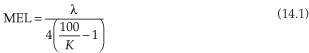
Misek, who may well be the leading proponent of the Beverage antenna, uses numbers like 1.6λ to 1.7λ over the 1.8- to 7.3-MHz region, and 0.53λ to 0.56λ on frequencies lower than 1.8 MHz. Dr. Beverage was once quoted as saying that the optimum length is 1λ. Perhaps the most important point to take away from this discussion is that the exact length is not critical. The author has employed Beverages of various lengths for over a quarter-century and has found little to recommend lengths in excess of 500 to 550 ft (1λ on 160 m) for use of frequencies between 1 and 7 MHz. Some of his current Beverages are in the 250- to 300-ft range; they have made it possible to pull weak stations out of the noise on 160 and 80 m on so many occasions it is hard to believe there is much improvement left to be gained by lengthening them. Of course, the longer a Beverage is, the narrower the main lobe—so in principle the greater the number of them you need to cover the compass rose.
Like the nonresonant longwire antenna, the Beverage needs a termination resistor that is connected to a good ground. This requirement is somewhat in conflict with the assumption that Beverage antennas work best over lossy ground, but the solution is to make a good artificial RF ground with radial wires at the terminated end. As in the longwire case, insulated or bare wires, at least 0.2λ long on the lowest frequency of interest, make the best radials. However, a substantial improvement in the ground is possible using wires only 15 to 20 ft in length (which is much less than λ/4 at the frequencies of interest), atop or just below the surface of the soil. Some experienced Beverage users recommend just one or two radials for each band, laid out at right angles to the Beverage wire itself. Bear in mind that while a ground rod driven into the earth at the terminating resistor makes a great mechanical tie point for joining the end of the Beverage to the resistor and any radials, it makes a lousy RF ground. The author has had good results (maybe not “perfect” results, but . . .) with two 0.1λ radials for each amateur band of interest, oriented at right angles to the Beverage wire itself. Wires in close proximity to ground—even lossy ground—should be thought of as providing nonresonant capacitive coupling rather than resonance, so their exact length is not important.
In addition to the radials and ground rod, Misek also recommends using a wire connection between the ground connection at the termination resistor and the ground connection at the receiver transformer. According to Misek, this wire helps to stabilize the impedance variations at higher frequencies.
The basic single-wire Beverage antenna of Fig. 14.1 consists of a single conductor (#18 to #8 wire gauges are most common) erected about 8 to 10 ft above ground. Because the RF power in a receiving Beverage is minuscule, the size and metallic composition of the wire are primarily set by mechanical (strength) and metallurgical (corrosion lifetime) considerations, rather than electrical. In contrast to most antennas, the greatest threat to Beverage longevity comes from dead trees and limbs falling on them or animals running into them. #14 THHN copper wire from building supply outlets is probably the most consistently economical source, although the antenna may have to be retensioned periodically. Some have used copper-clad steel or electric fence wire, but the author has found that the use of alternative metals or bimetallic wires often brings with it a new set of problems greater than the slight stretchiness of softdrawn copper wire.
Some Beverages are unterminated (and, hence, bidirectional), but most are terminated at one end in a resistance R equal to the antenna’s characteristic impedance, Z0. For the heights discussed, Z0 is likely to be between 300 and 800 Ω. The receiver end should also be terminated in its characteristic impedance, but ideally requires an impedance-matching transformer to reduce the antenna impedance to the 50-Ω or 75-Ω standard impedance used by most modern HF transceivers and receivers.
Installation of the Beverage antenna is not overly critical if certain rules are followed:
• For safety of humans and animals, install the antenna at a height of 8 to 10 ft above ground. Check its entire length frequently; because they are so low, Beverages have an annoying habit of collecting fallen branches or entire trees!
• Use a compass to run the Beverage wire in a reasonably straight line for the distance and beam heading you have selected. (The iPhone has a wonderful compass app that is free!) Typical Beverage lengths range from 250 to 1200 ft. If space permits, choose your Beverage location to maximize the distance between it and other low-band antennas, towers, power lines, buildings, and nearby sources of electrical noise (including your neighbor’s electrical heating pad and all the wall adapters in your own home as well as his).
• Support the wire as necessary (probably every 25 to 100 ft, depending on wire type). Beverages in the open can be mounted on treated 4 × 4 posts, but a potentially less expensive approach is to drive a few feet of an inexpensive steel rod (rebar, for instance) partway into the ground and drop an 8-ft length of PVC pipe over the rod. (Drill or slot the top of the PVC to hold the wire in place.)
• In wooded areas insulated wire can be draped over tree limbs of the appropriate height, or electric fence insulators obtained at farm supply stores can be nailed into the tree trunk. (Never wrap a wire or rope around a tree trunk or branch!) If the preferred path for your Beverage takes it between trees, run nylon twine between two trees straddling the desired path and hang the Beverage from the middle of the twine.
• Keep the wire a relatively constant height above ground. In other words, follow the slope of the terrain. The farther your Beverage wire is above ground, the less it is able to discriminate between desired low-angle signals and undesired higher-angle signals.
• Drop the vertical end sections straight down unless it’s more convenient to bring them down gradually through some horizontal distance.
• Drive a 6- or 8-ft ground rod at the termination end and attach one or two radials, 50 to 200 ft long, at right angles to the Beverage. The termination end is the end from which signals will be received. In other words, if the termination resistor is at the western end of a Beverage wire running east and west, the Beverage will favor signals coming from the west. Excellent 8-ft galvanized steel rods and mating brass clamps are available from many electrical supply stores and utility supply houses such as Graybar and others.
• Connect a termination resistor (see text below) from the bottom end of the drop wire at the termination end of the Beverage to a clamp on the ground rod there.
• Drive another ground rod and lay out a separate set of radials at the opposite end of the wire. This is the feedpoint of the Beverage.
If you have a junk box full of old resistors, a 470-Ω 2W carbon composition resistor makes a great Beverage termination. If you have only larger resistance values, connect two or more in parallel; the greater the installed wattage, the less susceptibility to damage from lightning-induced surges. The exact value of resistance is not critical, but the type of resistor is. Many of today’s resistors, especially the wire-wound ones, are not suitable for this application because they are intended for use in dc or audio circuits and exhibit too much inductive reactance at RF. A suitable alternative to carbon composition is a thick-film resistor, such as Ohmite’s TCH line.
Once your Beverage is installed, a good preliminary test is to measure the dc resistance between the unterminated drop wire and the ground rod at that end of the Beverage. With average ground characteristics, RTOTAL (the sum of the termination resistance plus the ground path between the meter and the grounded end of the termination) will probably range from 1.5 RTERM to 4RTERM, depending on the length of the Beverage and the characteristics of the ground beneath it. The primary value of this test is simply to prove continuity through the Beverage wire and termination resistor into the ground. This test should be performed when the installation is new, and the value of RTOTAL immediately recorded for future reference.
If you have the necessary test equipment, consider “sweeping” the impedance of the Beverage at its feedpoint over the frequency range of interest while you adjust the value of the terminating resistor for flattest response over the useful range. (Temporarily use a noninductive potentiometer in place of the permanent terminating resistor.) Make sure you terminate or match the feedpoint end of the Beverage according to the instructions with the test equipment. This is an excellent use of a vector network analyzer (VNA) of the type discussed in Chap. 27.
An inexpensive Beverage feedline is 75-Ω RG-6 coaxial cable purchased by the 500-or 1000-ft spool from a building supplies store.
When using either 50-Ω or 75-Ω coaxial cable for the feedline, a 9:1 step-down transformer at the Beverage feedpoint is a smart addition. (Do not put the transformer at the receiver end of the feedline!) Figure 14.3 shows how to build an appropriate transformer using a ferrite core and a trifilar winding. Type 31 or Type 43 materials should work well, but many mixes will work nearly as well. Ideally, the ground for the shield of the coaxial feedline at the transformer needs to be kept isolated from the grounded end (winding terminal a2 in Fig. 14.3) of the transformer winding that connects to the Beverage, which would require a second, completely isolated coaxial cable output winding identical to winding a1-a2 on the same core and a second “ground” terminal, but the author has three “very satisfactory” short Beverages (each 250 to 300 ft) with no ground isolation at all that provide excellent signal-to-noise enhancement on 160 and 80 m most nights.

FIGURE 14.3 Trifilar-wound 9:1 step-down Beverage transformer.
After connecting the feedline to the step-down transformer at the unterminated end of the Beverage, perform the same dc continuity test with an ohmmeter located at the receiver end of the feedline, thus checking the integrity of that portion of the signal path as well. Of course, you should see a very low value of R—no more than a few ohms, at most. The exact value will depend on the length of your feedline and the resistance of its conductors.
At this point, if a VNA or other suitable piece of test apparatus is available, a sweep of the entire antenna system from the receiver end of the feedline to the termination resistance at the far end of the Beverage wire can be an extremely valuable record should troubleshooting be necessary in the future.
Much has been learned and disseminated about the Beverage in the past decade. A book nearly as large as this one could be written about the antenna and all its subtleties and “picky details” that should be attended to. Nonetheless, “imperfectly” constructed Beverages can make a whole new layer of weak DX signals on the AM broadcast band or lower-frequency ham bands jump out of the background noise in your headphones. Yes, the author’s 250-ft Beverages are “too short” to be of much use on 160 m. Yes, the author’s Beverages should have matching transformers and isolated grounds. Etcetera, etcetera. But once the three most important compass headings were determined, each of the author’s Beverages took no more than two or three hours to install and connect. And they work on 160, 80, 40, and the AM broadcast band! Could they be fine-tuned to work better? Yep! Do they work well enough? Yep! Did they cost a lot? Nope! In short, the Beverage is the epitome of a practical antenna.
The Bidirectional Beverage
With some clever transformer “magic”, two Beverages, consisting of two parallel wires and capable of receiving from two separate compass headings 180 degrees apart, can share a common set of supports and a common feedline attached to the end of the wire pair that is nearer the receiver.
Figure 14.4 shows the circuit configuration that allows switching of the wires and the feedlines for two opposing directions. The parallel wires can be implemented in a variety of ways:

FIGURE 14.4 Two-wire reversible Beverage.
• Separate wires about a foot apart, supported by cross-arms atop wood or PVC supports
• Open-wire transmission line
• Two-conductor jacketed house wiring
• Surplus multiconductor cable
Transformers T1 and T2 are designed to transform the Beverage impedance down to the characteristic impedance, Z0, of the coaxial feedline to the receiver. In operation, one of the two coaxial cables feeds the receiver while the other cable must be terminated in Z0. This can be done at the receiver end, but, alternatively, to avoid running two transmission lines to the receiver, the resistive load switching and swapping of transformers feeding the receiver can be performed in a protective enclosure near the end of the Beverage that is attached to transformer T1. In the latter configuration, the dc control signal to switch a multipole double-throw relay in the enclosure can be multiplexed on the coaxial cable.
Assume first that the feedline attached to transformer T1 is terminated in Z0. Signals coming from the right side of the page build in voltage with respect to ground along both Beverage wires equally. At the left end of the wires, this common mode voltage appears across the entire primary winding of T1, including its centertap, and drives the top end of the primary winding of T2, whose secondary feeds the active coaxial cable to the receiver. Signals coming from the left side of the page build up equally on both Beverage wires from left to right, appearing on the entire primary of T3, including its centertap, which drives one end of a secondary winding. The signal across the secondary of transformer T3 now drives the two Beverage wires in push-pull or differential mode, and that signal propagates from right to left along the wires until it reaches the primary of T1, where it is coupled to the secondary and dissipated in that winding’s Z0 termination. To receive signals from the opposite direction, the receiver is connected to the secondary of T1, and the secondary of T2 is terminated in Z0.
The exact number of turns required on each transformer is dependent upon the specifics of each individual Beverage installation, including wire diameter and length, spacing between the two wires, height above ground, and ground conductivity. If the termination and cable switching is done near T1 and T2, care must be taken to isolate the ground end of the termination from the coaxial cable ground (through a separate pole on the relay), or the ground connecting the two must be virtually perfect.
Phased Beverages
Additional directivity and signal amplitude can be obtained by phasing two or more Beverages. At least two different methods of phasing are currently in use:
• Two identical Beverages, parallel to each other, spaced λ/4 or more apart, with no offset relative to the desired receiving direction. (That is, they can be thought of as two opposing long sides of a rectangle.) The outputs of the two wires are combined in phase before reaching the receiver.
• Two identical Beverages, parallel to each other and closely spaced (i.e., within a few feet), but offset somewhat in the desired receiving direction. (Similarly, picture the long sides of a very skinny parallelogram.)
A Beverage erected with two wires—parallel to each other, at the same height, spaced about 12 in apart (Fig. 14.5), with a length that is a multiple of a half-wavelength—is capable of null steering. That is, the rear null in the pattern can be steered over a range of 40 to 60 degrees. This feature allows strong, off-axis signals to be reduced in amplitude so that weaker signals in the main lobe of the pattern can be received. There are at least two varieties of the steerable wave Beverage (SWB).

FIGURE 14.5 Beverage antenna with a steerable null.
If null steering behavior is desired, then a phase control circuit (PCC) will be required—consisting of a potentiometer, an inductance, and a variable capacitor all connected in series. Varying both the “pot” and the capacitor will steer the null. The direction of reception and the direction of the null can be selected by using a switch to swap the receiver and the PCC between port A and port B.
Snake or BOG Antenna
The height above ground of a Beverage is the result of a compromise that invariably includes a need to locate the antenna high enough to avoid damage to or from humans and animals. As a result, the rejection of signals from undesired directions and signals with horizontal polarization is lessened.
The Beverage on ground (BOG) or snake antenna attempts to minimize unwanted signal ingress by eliminating the vertical downlead at each end of the Beverage. A side benefit is the elimination of all supports! The primary disadvantage is a noticeable reduction in received signal level stemming from the very close coupling of the antenna to the ground beneath it. Typically, a preamplifier must be added to a BOG or snake in order to develop signal levels sufficient to override the receiver noise floor. Ideally the preamp should be located at the junction of the Beverage and its feedline, rather than at the receiver end of the feedline.
Receiving Loops
Even in their smallest implementations, the preceding antennas require a fair amount of real estate for their proper operation. In addition to the space taken up by the antenna itself, there is a “hidden” requirement of another λ/2 or more distance between the receiving antenna and any transmitting antennas resonant on the same band(s). Further, it is wise to locate and orient Beverages so as to keep buildings containing computers, microprocessors, and other sources of RF noise behind the antenna—i.e., at the receiver, or unterminated, end. In general, a broadcast-band listener (BCL) or shortwave listener (SWL) contemplating the installation of Beverages for multiple compass headings will need a 10-acre or larger parcel.
Two entirely different classes of antenna have been of great use to listeners with limited space for antennas. The first of these is the traditional small, multiturn loop that has been around for years. The second is a whole new class of small, single-turn loops that emulate the directivity of large transmitting loops while exploiting size reduction design techniques uniquely available to receiving antennas that do not need to exhibit RF efficiency.
Small Loop Receiving Antennas
Radio direction finders and people who listen to the AM broadcasting bands, VLF, medium-wave, or the so-called low-frequency tropical bands are all candidates for a small loop antenna. These antennas are fundamentally different from the large (transmitting) loops of Chap. 7 and the multielement versions of Chap. 13. Large loop antennas typically have a total wire length of 0.5λ or greater. Small loop antennas, on the other hand, have an overall total conductor length that is less than about 0.1λ.
Earlier in this book we talked about the importance of proper physical configuration to efficient performance as a radiating antenna by a conductor. In particular, we pointed out that a half-wavelength of copper wire that is wound into a tight coil is a poor antenna and is best treated as a lumped-circuit inductor. Now we go a step further and note that a small loop antenna responds to the magnetic field component of the electromagnetic wave instead of the electrical field component. (Remember from high school science class that passing a bar magnet back and forth rapidly through the interior of a multiturn coil produces temporary voltages across the terminals of the coil. Consider the time-varying magnetic field in a transmitted wave as analogous to the movement of the bar magnet.)
Thus we see a principal difference between a large loop (total conductor length greater than 0.1λ) and a small loop when examining the RF currents induced in either loop when a signal intercepts it. In a large loop, the current is a standing wave that varies (sinusoidally) from one point in the conductor to another, much like a dipole, and we analyze its operation in much the same way we have examined dipoles; in the small loop antenna, the current is the same throughout the entire loop.
Since the electric and magnetic fields of a radiated wave in free space are at right angles to each other and to the direction the wave propagates through space, and since we are primarily listening for vertically polarized signals with loops, the magnetic field is oriented horizontally, or nearly so.
The differences between small loops and large loops show up in some interesting ways, but perhaps the most striking difference is found in the directions of maximum response—the main lobes—and the directions of the nulls. Both types of loops produce figure eight patterns but at right angles with respect to each other. The large loop antenna produces main lobes that are orthogonal—i.e., at right angles or “broadside”— to the plane of the loop. Nulls are off the sides of the loop. The small loop, however, is exactly the opposite: the main lobes are off the sides of the loop (in the plane of the loop), and the nulls are broadside to the loop plane (Fig. 14.6A). Do not confuse small loop behavior with the behavior of the loopstick antenna. Loopstick antennas are made of coils of wire wound on a ferrite or powdered-iron rod. The direction of maximum response for the loopstick antenna is broadside to the rod, with deep nulls off the ends (Fig. 14.6B). Both loopsticks and small wire loops are used for radio direction-finding and for shortwave, low-frequency medium-wave, AM broadcast band, and VLF listening.
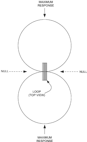
FIGURE 14.6A Small loop antenna.

FIGURE 14.6B Loopstick antenna.
The nulls of a loop antenna are very sharp and very deep. If you point a loop antenna so that its null is aimed at a strong station, the signal strength of the station appears to drop dramatically at the center of the notch. Turn the antenna only a few degrees one way or the other, however, and the signal strength increases sharply. The depth of the null can reach 10 to 15 dB on sloppily constructed loops and 30 to 40 dB on well-built units (30 dB is a very common value), and there have been claims of 60-dB nulls for some commercially available loop antennas. The construction and uniformity of the loop are primary factors in the sharpness and depth of the null.
Radio direction-finding (RDF) has long been a major application for the small loop antenna, especially in the lower-frequency bands. Chapter 24 is devoted to the use of loops and other antenna types specifically for RDF purposes.
Today, the use of these small loops has been extended into the general receiving arena, especially on the low frequencies (VLF through lower HF range). In this application they are often physically quite large (compared, for instance, to the receiver they are apt to be used with) and require many turns of wire to develop the necessary signal amplitudes and notch depth. Receiving loops have also been used as high as VHF and are commonly used in the 10-m ham band for hidden transmitter hunts.
Let’s examine the basic theory of small loop antennas and then take a look at some practical construction methods.
Grover’s Equation
Grover’s equation (Grover, 1946) seems closer to the actual inductance measured in empirical tests than certain other equations that are in use. This equation is
![]()

K1 through K4 are shape constants and are given in Table 14.1. ln is the natural logarithm of this portion of the equation; it is typically obtained from a table or scientific calculator. (See App. A for information on natural logarithms.)

Air Core Frame (“Box”) Loops
A wire loop antenna is made by winding a large coil of wire, consisting of one or more turns, on some sort of frame. The shape of the loop can be circular, square, triangular, hexagonal, or octagonal, but for practical construction reasons the square loop is most popular. With one exception, the loops considered in this section will be square, so you can easily duplicate them.
The basic form of the simplest loop, as shown in Fig. 14.7, is square, with sides of length A. The width of the loop (B) is the distance from the first turn to the last turn in the loop or, alternatively, the diameter of the wire if only one turn is used. The turns of the loop in Fig. 14.7 are depth-wound—meaning that each turn of the loop is spaced in a slightly different parallel plane—and spaced evenly across distance B. Alternatively, the loop can be wound such that the turns are in the same plane (known as planar winding). In either case, the sides of the loop (A) should be not less than five times the width (B). There seems to be little difference in performance between depth- and planar-wound loops: the far-field patterns of the different shape loops are nearly the same if the respective cross-sectional areas (πr2 for circular loops and A2 for square loops) are less than λ2/100.
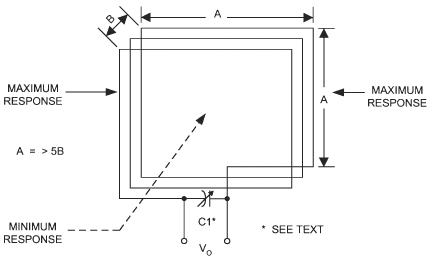
FIGURE 14.7 Simple loop antenna.
The reason a small loop has a null when its broadest aspect is facing the signal is simple, even though it seems counterintuitive at first blush. In Fig. 14.8 we have two identical small loop antennas at right angles to each other. Antenna A is in line with the advancing radio wave, whereas antenna B is broadside to the wave. Each line in the wave represents a line where the signal strength is the same, i.e., an isopotential line. When the loop is in line with the signal (antenna A), a difference of potential exists from one end of the loop to the other and current can be induced in the wires. When the loop is turned broadside, however, all points on the loop are on the same potential line, so there is no difference of potential between segments of the conductor. Thus, little signal is picked up (and the antenna therefore sees a null).

FIGURE 14.8 Two small loop antennas at right angles to each other.
The actual voltage across the output terminals of an untuned loop is a function of the angle of arrival of the signal α (Fig. 14.9), as well as the strength of the signal and the design of the loop. The voltage Vo is given by
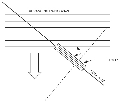
FIGURE 14.9 Untuned loop antenna at an angle to received wave.
![]()

Loops are sometimes specified in terms of the effective height of the antenna. This number is a theoretical construct that compares the output voltage of a small loop with a vertical segment of identical wire that has a height of
![]()
If a capacitor (such as C1 in Fig. 14.7) is used to tune the loop, then the output voltage Vo will rise substantially. The output voltage found using the first equation is multiplied by the loaded Q of the tuned circuit, which can be from 50 to 100:
![]()
Even though the output signal voltage of tuned loops is higher than that of untuned loops, it is nonetheless low compared with other forms of antenna. As a result, a loop preamplifier usually is needed for best performance.
Transformer Loops
It is common practice to make a small loop antenna with two loops rather than just one. Figure 14.10 shows such a transformer loop antenna. The main loop is built exactly as previously discussed: several turns of wire on a large frame, with a tuning capacitor to resonate it to the frequency of choice. The other loop is a one- or two-turn coupling loop. This loop is installed in very close proximity to the main loop, usually (but not necessarily) on the inside edge, not more than a couple of centimeters away. The purpose of this loop is to couple signal induced from the main loop to the receiver at a more reasonable impedance match.
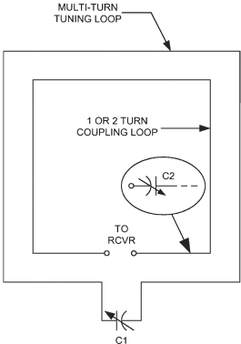
FIGURE 14.10 Transformer loop antenna.
The coupling loop is usually untuned, but in some designs a tuning capacitor (C2) is placed in series with the coupling loop. Because there are many fewer turns on the coupling loop than on the main loop, its inductance is considerably smaller. As a result, the capacitance to resonate is usually much larger. In several loop antennas constructed for purposes of researching this chapter, the author found that a 15-turn main loop resonated in the AM BCB with a standard 365-pF capacitor, but the two-turn coupling loop required three sections of a ganged 3 × 365-pF capacitor connected in parallel to resonate at the same frequencies.
In several experiments, the loop turns were made from computer ribbon cable. This type of cable consists of anywhere from 8 to 64 parallel insulated conductors arranged in a flat ribbon shape. Properly interconnected, the conductors of the ribbon cable form a continuous loop. It is no problem to take the outermost one or two conductors on one side of the wire array and use them for a coupling loop.
Tuning Schemes for Loop Antennas
Loop performance is greatly enhanced by tuning the inductance of the loop to the desired frequency. The bandwidth of the loop is reduced, which reduces front-end overload from strong off-frequency signals. Tuning also increases the signal level available to the receiver by a factor of 20 to 100 times. Although tuning can be a bother if the loop is installed remotely from the receiver, the benefits are well worth it in most cases.
Various techniques for tuning are detailed in Fig. 14.11. The parallel tuning scheme, which is by far the most popular, is shown in Fig. 14.11A. In this type of circuit, the capacitor (C1) is connected in parallel with the inductor, which in this case is the loop. Parallel-resonant circuits present a very high impedance to signals on their resonant frequency and a very low impedance to other frequencies. As a result, the voltage level of resonant signals is very much larger than the voltage level of off-frequency signals.
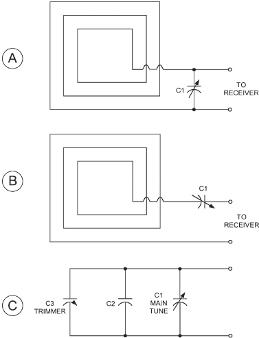
FIGURE 14.11 Various tuning schemes. (A) Parallel. (B) Series resonant. (C) Series or parallel.
The series-resonant scheme is shown in Fig. 14.11B. In this circuit, the loop is connected in series with the capacitor. Series-resonant circuits offer a high impedance to all frequencies except the resonant frequency (exactly the opposite of the case of parallel-resonant circuits). As a result, current from the signal will pass through the series-resonant circuit at the resonant frequency, but off-frequency signals are blocked by the high impedance.
There is a wide margin for error in the inductance of loop antennas, and even the complex equations that appear to provide precise values of capacitance and inductance for proper tuning are only estimates. The exact geometry of the loop “as built” determines the actual inductance in each particular unit. As a result, it is often the case that the tuning provided by the capacitor is not as exact as desired, so some form of compensation is needed. In some cases, the capacitance required for resonance is not easily available in a standard variable capacitor, and some means must be provided for changing the capacitance. Figure 14.11C shows how this is done. The main tuning capacitor can be connected in either series or parallel with other capacitors to fine-tune the overall value. If the capacitors are connected in parallel, the total capacitance is increased (all capacitances are added together). If the extra capacitor is connected in series, however, then the total capacitance is reduced. The extra capacitors can be switched in and out of a circuit to change frequency bands.
Tuning of a remote loop can be a bother if it is done by hand, so some means must be found to do it from the receiver location (unless you enjoy climbing into the attic or onto the roof). Traditional means of tuning called for using a low-rpm dc motor, or stepper motor, to turn the tuning capacitor. Once upon a time, the little 1- to 12-rpm motor used to drive rotating displays in retail store show windows was popular. But this approach is not really needed since the advent of varactors.
A varactor is a reverse-biased diode whose junction capacitance is a strong function of the applied dc bias voltage. A high voltage (such as 30 V) drops the capacitance, whereas a low voltage increases it. Varactors are available with maximum capacitances of 22, 33, 60, 100, and 400 pF. The latter are of great interest to us for this application because they have the same range as the tuning capacitors normally used with loops.
Figure 14.12 is the schematic of a remote tuning system for loop antennas. The tuning capacitor is a combination of a varactor diode plus two optional capacitors: a fixed capacitor (C1) and a trimmer (C2). The dc tuning voltage (VT) is provided from a fixed dc power supply (V+) located at the receiver end. A potentiometer (R1) is used to tune the loop by setting the voltage going to the varactor. A dc blocking capacitor (C3) keeps the dc tuning voltage from being shorted out by the receiver input circuitry.
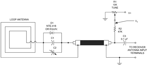
FIGURE 14.12 Remote tuning scheme using varactor diode.
The Sports Fan’s Loop
Okay, sports fans, what do you do when the best game of the week is broadcast only on a low-powered AM station and you live at the outer edge of their service area, where the signal strength leaves much to be desired? You use the sports fan’s loop antenna, that’s what! The author first learned of this antenna from a friend—a professional broadcast engineer who worked at a religious radio station that had a pipsqueak signal but lots of fans. It really works; in fact, one might say it’s a “miracle”.
The basic idea is to build a 16-turn, 60-cm2 tuned loop and then place the AM portable radio at the center with its loopstick aimed so that its null end is broadside of the loop. When you do so, the nulls of both the loop and the loopstick are in the same direction. The signal will be picked up by the loop and then coupled to the radio’s loopstick antenna. Sixteen-conductor ribbon cable can be used for making the loop. For an extra touch of class, place the antenna and radio assembly on a dining room table lazy Susan to make rotation easier. A 365-pF tuning capacitor is used to resonate the loop. If you listen to only one frequency, this capacitor can be a trimmer type.
Shielded Loop Antennas
The loop antennas discussed thus far in this chapter have all been unshielded types. Unshielded loops work well under most circumstances, but in some cases their pattern is distorted by interaction with the ground and nearby structures (trees, buildings, etc.). In the author’s tests, trips to a nearby field proved necessary to measure the depth of the null because of interaction with the aluminum siding on his house. Figure 14.13 shows two situations. In Fig. 14.13A we see the pattern of the normal free-space loop, i.e., a perfect figure eight pattern. When the loop interacts with the nearby environment, however, the pattern distorts. In Fig. 14.13B we see some filling of the notch for a moderately distorted pattern. Some interactions are so severe that the pattern is distorted beyond all recognition.
FIGURE 14.13A Normal free-space loop.
FIGURE 14.13B Filling of the notch.
Interaction can be reduced by shielding the loop, as in Fig. 14.14. Loop antennas operate on the magnetic component of the electromagnetic wave, so the loop can be shielded against E-field signals and electrostatic interactions. In order to retain the ability to pick up the magnetic field, a gap is left in the shield at one point.

FIGURE 14.14 Shielding the loop.
There are several ways to shield a loop. You can, for example, wrap the loop in adhesive-backed copper-foil tape. Alternatively, you can wrap the loop in aluminum foil and hold it together with tape. Another method is to insert the loop inside a copper or aluminum tubing frame. Or . . . the list seems endless.
Sharpening the Loop
Many years ago, the Q-multiplier was a popular add-on accessory for a communications receiver. These devices could be found in certain receivers (the National NC-125 from the 1950s comes to mind) or offered as an outboard receiver accessory by Heathkit, and many construction projects could be found in magazines and amateur radio books. The Q-multiplier improves receiver performance by increasing the sensitivity and reducing the bandwidth of certain receiver stages.
The Q-multiplier of Fig. 14.15 is an active electronic circuit placed at the antenna input of a receiver. It is essentially an Armstrong oscillator that does not quite oscillate. These circuits have a tuned circuit (L1/C1) at the input of an amplifier stage and a feed-back coupling loop (L3). The degree of feedback is controlled by the coupling between L1 and L3. The coupling is varied by changing both how close the two coils are and their relative orientation with respect to each other. Certain other circuits use a series potentiometer in the L3 side that controls the amount of feedback.

The Q-multiplier is adjusted to the point that the circuit is just on the verge of oscillating. As the feedback is backed away from the threshold of oscillation—but not too far—the bandwidth narrows and the sensitivity increases. It takes some skill to operate a Q-multiplier, but it is easy to use once you get the hang of it and is a terrific accessory for any loop antenna.
Loop Amplifier
Figure 14.16 shows the circuit for a practical loop amplifier that can be used with either shielded or unshielded loop antennas. It is based on junction field-effect transistors (JFETs) connected in cascade. The standard common-drain configuration is used for each transistor, so the signals are taken from the source terminals. The drain terminals are connected together and powered from the +12V dc power supply. A 2.2-µF bypass capacitor is used to put the drain terminals of Q1 and Q2 at ground potential for ac signals while keeping the dc voltage from being shorted out.
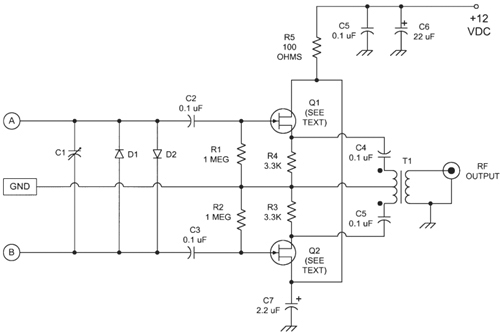
FIGURE 14.16 Practical loop amplifier.
The two output signals are applied to the primary of a transformer, the centertap of which is grounded. To keep the dc on the source terminals from being shorted through the transformer winding, a pair of blocking capacitors (C4, C5) is used.
Input signals are applied to the gate terminals of Q1 and Q2 through dc blocking capacitors C2 and C3. A pair of diodes (D1, D2) keeps high-amplitude noise transients from affecting the operation of the amplifier. They are connected back to back in order to snub out both polarities of signal.
Tuning capacitor C1 is used in lieu of a capacitor in the loop; it resonates the loop at a specific frequency. Its value can be found from the equation given earlier.
The transistors used for the push-pull amplifier (Q1, Q2) can be nearly any general-purpose JFET device (MPF-102, MPF-104, etc.). A practical approach for many people is to use transistors from service replacement lines, such as the NTE-312 and NTE-316 devices.
Special Problem for VLF/LF Loops
A capacitance is formed whenever two conductors are side by side. A coil exhibits capacitance as well as inductance because the turns are side by side. Unfortunately, with large multiturn loops, this capacitance can be quite large. The distributed capacitance of the loop self-resonates with the inductance. Loop antennas do not work well at frequencies above their self-resonant frequency, so it is sometimes important to raise the self-resonance to where it does not affect operation at the desired frequencies.
Figure 14.17 shows one way to raise the self-resonant point. The turns on the loop are broken into two or more groups separated by spaces. This method reduces the effective capacitance by placing the capacitances of each group of wires in series with the others. The effective capacitance of a series string of capacitors is always less than the value of the smallest capacitor.

FIGURE 14.17 Raising the self-resonant frequency.
![]()
Coaxial-Cable Loop Antennas
One of the more effective ways to make a shielded loop is to use coaxial cable. Figure 14.18 shows the circuit of such a loop. Although only a single-turn loop is shown, there can be any number of turns. One reader made a 100-kHz LORAN (a navigation system) loop using eight turns of RG-59/U coaxial cable wound with an 8-ft diameter.

FIGURE 14.18 Coaxial-cable shielded loop.
Note the special way that the coaxial cable is connected. This method is called the Faraday connection after the fact that the shield of the coax forms a Faraday shield. At the output end, the center conductor of the coaxial cable is connected to the center conductor of the coaxial connector, and the cable shield is connected to the connector ground/shield terminal. At the other end of the loop, the shield is left floating, but the center conductor is connected to the shield at the connector end, not at any other point.
The EWE Antenna
In 1995 Floyd Koonce, WA2VWL, published details of his EWE antenna, which provides MF and low HF receiving directivity in a much smaller footprint than a Beverage antenna. The acronym EWE is not only descriptive (Earth-Wire-Earth) but a play on words, as well, since the antenna has the shape of an inverted “U” (in response to which the author can only say “Bah!”).
The EWE of Fig. 14.19 functions much as if it were a two-element phased array of short verticals. However, like the Beverage, the EWE is a traveling wave antenna. Directivity is a result of phase and amplitude differences between the two vertical segments; these differences, in turn, originate in the length of the horizontal wire connecting the vertical runs, the value of the termination resistor, and the fact that a current flowing upward in one vertical segment flows downward in the other.

Unlike the Beverage, the EWE receives from the end of the antenna opposite the termination resistor. Because the antenna is not a resonant device, it is relatively broadband in operation, although the optimum value of termination resistance varies with frequency (and with the exact characteristics of the ground beneath the antenna). The value of the termination is best set by tuning for a null off the back of the antenna by listening to appropriate stations in the AM broadcast band or on 160 m. Typical values for the termination resistor are in the 700- to 900-Ω range. The input impedance is somewhat lower and is a reasonably good match to 50-Ω coax and receiver inputs via a 9:1 transformer.
Although the EWE requires a much smaller space than a Beverage antenna, to achieve its full potential it needs to be kept away from other conductors. This constraint can substantially increase the actual space required by the EWE.
Pennants, Flags, and the K9AY Loop
The appearance of the EWE inspired other experimentally inclined radio amateurs to develop additional low-band receiving antennas for small spaces. Subsequent to publication of the EWE, at least three new single-turn terminated loop designs came into being. As is the case with the EWE, for those lacking the necessary space for a set of Beverage antennas, these loops provide an alternative, although those fortunate enough to have the space for both generally report hearing a little bit better with their Beverages.
Directivity of this family of loops is based on constructive versus destructive combining of the E- and H-fields that constitute an arriving radio wave. An arriving E-field in the plane of the loop induces a voltage in the loop just as it would in any other short (relative to wavelength) wire. The associated H-field at right angles to the loop plane induces a current in the loop that becomes a voltage across the terminating resistor. When these fields arrive from one direction, the two voltages sum; when arriving from the opposite direction, they subtract.
Figure 14.20 depicts the K9AY terminated loop. Exact shape of the loop is not critical, but the bottom leg must come near earth for the termination and transformer ground connections. The total length of wire in the loop is about 85 ft, and a single support only 25 ft tall is required. The feedpoint impedance is similar to that of a typical Beverage, so a 9:1 transformer is required. Like the EWE and unlike the Beverage, however, the direction of maximum signal pickup is opposite the terminated end.

The pattern of the K9AY loop is unidirectional. By using relays to switch the termination and feedpoint, one loop can be switched between two opposing directions. Two loops, at right angles to each other and similarly switched, can provide four directions from a single fixed mast.
Like the other members of the pennant and flag family, the K9AY loop is quite sensitive to detuning from nearby conductors. As a result, some of its impressive space savings are not always fully realizable if the user also has transmitting antennas and towers nearby. Proper operation of the K9AY is fairly sensitive to the exact value of the termination resistor and depends on both the operating frequency and the actual characteristics of the ground beneath the antenna. Many implementations use a remotely controlled termination resistor to optimize the depth of the null to the rear as the received frequency is changed and to compensate for seasonal variations in soil characteristics.
In many operating scenarios, the value of this antenna is likely to be more for its null off the rear than for any forward directivity it exhibits. But that’s quite appropriate for much of the weak-signal work that occurs on the 160- and 80-m amateur bands, or when broadcast band DXing.
The pennant (Fig. 14.21A) was developed by Jose Mata, EA3VY, and Earl Cunningham, then-K6SE (deceased), to overcome the EWE’s sensitivity to the characteristics of the ground beneath it. The resulting pennant design exhibits stability of pattern and performance over a wide variety of grounds and can be raised (on a mast) to a wide range of heights. The favored design also tweaks dimensions and terminating resistor value to arrive at a purely resistive feedpoint impedance for optimum matching with a 9:1 transformer.

FIGURE 14.21A Pennant antenna.
Just as the pennant is a triangular receiving antenna, the flag (Fig. 14.21B) is a rectangular one. Because the capture area of a flag is somewhat larger than that of a pennant, the flag antenna provides somewhat greater output voltage to the feedline for a given signal than does the pennant.

Unlike the Beverage, all these antennas receive away from the terminating resistor. All must be mounted on, or supported by, nonmetallic members (such as PVC pipe) and must not be located near any metallic structures—especially those having dimensions in the vertical plane that are a sizeable fraction of a wavelength at LF through lower HF frequencies—unless steps are taken to detune those structures at the frequencies of interest while receiving.
Many amateurs and BCLs have employed multiple phased pennants and flags to obtain even greater improvements in received signal-to-noise ratio. An Internet search on these antenna types will return many detailed and useful references.
Longwire Antennas
No discussion of HF receiving antennas would be complete without mention of the longwire antenna. This is often the first external antenna ever used by a broadcast band DXer or SWL. Its primary attribute is simplicity. Its primary disadvantage is that it has a pattern that is either unpredictable or shifts from broadside to axial with increasing frequency. However, the beauty of this antenna is that if it is at least 100 ft long, it can provide hours of enjoyable listening to anything from VLF airport beacons through the AM broadcast band and on up into the amateur and international shortwave broadcast bands. The author has even used a longwire with receivers (such as small portables) that had no provision for connecting to an external antenna. Simply bring the end of the longwire near the receiver—perhaps wrapping it around the receiver enclosure a few turns.
Unfortunately, that same “one size fits all” versatility means the longwire rejects nothing, and strong off-frequency signals can overload just about any receiver unless some form of selectivity is applied at its front end. Even a high-end receiver will benefit from having a low-power antenna tuner (ATU) inserted in the path between it and a longwire antenna.
The longwire antenna is covered at length in Chap. 8 (“Multiband and Tunable Wire Antennas”) as a transmitting antenna, but some of the installation considerations there are of little importance for a receive-only installation. In particular, when used for transmitting a longwire must be operated against a good RF ground system, but if used only for receiving, the grounds associated with the receiver’s power cord are probably sufficient at all but the highest frequencies.
Because the longwire enters the structure where the receiver is located, it tends to faithfully pick up signals from any of the incidental radiators nearby: wall adapters, Ethernet circuits, computer power supplies, etc. In today’s electromagnetic environment, this may turn out to be its greatest shortcoming.