CHAPTER 8
Multiband and Tunable Wire Antennas
Most communications operators require more than one band, and that makes the antenna problem exactly that—a problem to be solved. Amateur, commercial, and military operators are especially likely to need either multiple antennas for different bands or a multiband antenna that operates on any number of different bands. This situation is especially likely on the high-frequency (HF) bands from 3.5 to 29.7 MHz.
Another problem regards the tunability of an antenna. Some amateur bands are very wide (several hundred kilohertz), and that causes the feedpoint impedance of most antennas to be highly variable from one end of the band to the other. It is typical for amateurs to design an antenna for the portion of the band that they use most often and then tolerate a high voltage standing wave ratio (VSWR) at the other frequencies. Unfortunately, when you see an antenna that seems to offer a low VSWR over such a wide range, it is almost certain that this broad response is the result of resistive losses that are reducing the antenna efficiency. However, it is possible to tune an antenna over a wide bandwidth using an adjustable antenna tuning unit (ATU) similar to those described in Chap. 24.
Multiband Antennas
For users whose interest (or license) is limited to narrow frequency ranges at a number of different places in the frequency spectrum, multiband antennas provide a reasonable approach to putting a good signal out on each of the desired bands. The sections that follow provide examples of some time-tested ways to do this.
Trap Dipoles
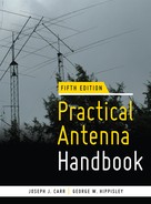
Perhaps the most common form of multiband wire antenna is the trap dipole shown in Fig. 8.1A. In this antenna category, parallel resonant traps are used in combination with shortened segments of wire or aluminum tubing to provide the equivalent of quarter-wavelength half-elements on each band of interest. The technique can be applied to monopoles or to both sides of a dipole or other balanced antenna. Typically, each trap is parallel resonant at one of the desired operating frequency ranges. The high impedance associated with a parallel-resonant circuit allows very little radiofrequency (RF) energy at the trap frequency to pass from one side of the trap to the other. At frequencies other than the trap design frequency, the RF excitation of the element passes through the trap relatively unattenuated. Below the trap design frequency, the trap appears as a net inductive component and above the design frequency it appears as a net capacitive component.
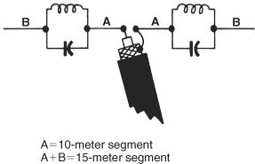
FIGURE 8.1A Trap dipole for multiband operation. (Courtesy of Hands-On Electronics and Popular Electronics)
Let’s look at how one pair of traps can provide two-band operation with low SWR for a simple dipole. In the example of Fig. 8.1A, the trap on each side of the center insulator is parallel resonant on 10 m. Because of the high impedance of the trap on that band, very little 10-m energy gets beyond the traps, and only the sections of wire labeled “A” have any appreciable RF in them. If the length of each section A is approximately one quarter-wavelength (or about 8 ft long on the 10-m band), the antenna will function as a resonant 10-m dipole on that band.
If a transmitted signal on a lower frequency (say, 15 m) is applied across the center of this antenna, the reactance of the trap capacitor will increase but the reactance of the inductor will decrease. Since the capacitor and the inductor are in parallel, the capacitor will not have a major impact on the operation of the antenna on 15 m, but the inductor will provide a modest amount of lumped-element “loading”. As a result, the sum of the lengths of A and B will be less than a full λ/4 (the natural nontrap length) on 15 m.
In general, trap dipoles are shorter than nontrap dipoles cut for the same band. The actual amount of shortening depends upon the values of the components in the traps, so consult the manufacturer’s data for each model of trap purchased.
Some trap antennas employ multiple traps on each side of the center insulator to cover three or more bands with a single feedline. The most popular combinations are probably 20-15-10 and 80-40-20, employing two separate parallel-resonant traps on each side of the insulator. The principle of operation is as previously described, except that a third wire segment is usually found between the two sets of traps on a side. Where more than one pair of traps is used in the antenna, make sure they are of the same brand and are intended to work together.
On all bands except the highest one, the radiation efficiency of the trap antenna will be somewhat less than that of a full λ/4 monopole or λ/2 dipole for the same band. That is because a small portion of the radiating element has been converted to a nonradiating lumped inductance. However, the effect is small, usually resulting in a net reduction in radiated field strength of 0.5 dB or so, depending on the exact design of the traps and their distance from the feedpoint.
A disadvantage of trap antennas is that they provide less harmonic rejection than an antenna designed for a single band. The antenna has no idea what band the transmitter “thinks” it’s transmitting on, so any harmonic energy that falls within any of the design bands of the trap antenna will be radiated with the same efficiency. As a result, users of multiband antennas need to take every reasonable precaution to be sure that harmonics and other out-of-band spurious emissions from their transmitters or transceivers and associated amplifiers are as low as possible.
Multiple Dipoles
Another approach to multiband operation of an antenna consists of two or more λ/2 dipoles fed from a single transmission line, as shown in Fig. 8.1B. There is no theoretical limit to how many dipoles can be accommodated, although there is certainly a practical limit based on the total weight of multiple dipoles and their spacers. One trick is to remember that bands related to each other by a 3:1 ratio of frequencies can probably be covered by a single dipole cut for the lower-frequency band. Such is the case, for instance, with 40 and 15 m and possibly even with 80 and 30 m.

FIGURE 8.1B Multiband dipole consists of several dipoles fed from a common feedline.
Assuming the dipoles are at least λ/2 above ground at the lowest frequency, a reasonably good match to the feedpoint impedance is provided by either 50-Ω or 75-Ω coaxial cable. The two sides of the coax (center conductor and shield) can be connected to the center of the multi-dipole directly or through a 1:1 balun transformer, as shown in Fig. 8.1B. Each antenna (A-A, B-B, or C-C) is cut to λ/2 at its design frequency, so the approximate overall length of each dipole can be found from the standard expression for dipole length.
Overall length (A + A, B + B, or C + C):
![]()
or, for each side of the dipole (A, B, or C):
![]()
As always, close to the earth’s surface these equations are approximations and are not to be taken too literally. Some experimentation will probably be necessary to optimize resonance on each band. Also, be aware that the drooping dipoles (B and C in this case) may act more like an inverted-vee antenna (see Chap. 6) than a straight dipole, so the equation length will be just a few percent too short. In any event, a little “spritzing” with this antenna will yield acceptable results.
Some amateurs build the multiple-band dipole from four- or five-wire flat TV rotator cable. Starting with the highest frequency, cut each wire to the required length and strip off any unused portions.
Another possibility is the “jumper-tuned” inverted-vee shown in Fig. 8.1C. In this situation, a single conductor, broken into segments A, B, and C (or more, if desired), is used for each leg of the antenna. Adjacent segments are separated by inline insulators. (Standard end insulators are suitable.) Segment A is a quarter-wavelength on the highest-frequency band of operation, A + B is a quarter-wavelength on the next highest band of operation, and A + B + C is a quarter-wavelength on the lowest-frequency band of operation.
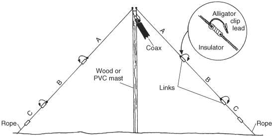
FIGURE 8.1C Multiband inverted-vee uses shorting links to change bands.
The antenna is “tuned” to a specific band by either connecting or disconnecting a wire (see inset) jumper across the insulator between the segments. Either a switch or an alligator clip jumper will short out the insulator to effectively lengthen the antenna for a lower band.
A big disadvantage to this type of multiband antenna is that you must go outside and manually switch the jumpers to change bands, which probably explains why other antennas are a lot more popular, especially in northern latitudes. One way to get at the higher jumpers is to make the center support a tilt-over mechanism (as described in Chap. 28).
Log-Periodic
From a distance, the log-periodic (LP) antenna resembles a long boom Yagi (Chap. 12) parasitic array, but it is not. Rather, it is an all-driven array that derives its name from the fact that each element length and the spacing from that element to the next one is a constant percentage of the previous element’s length and spacing, respectively. An open-wire parallel transmission line that runs the length of the boom feeds the centers of all elements, which are split and insulated at their midpoints, but the transmission line is flipped as it passes from element to element so that each element is fed 180 degrees out of phase with respect to the ones on either side of it. A commonly seen example of log-periodics is the modern multichannel VHF TV antenna, but much larger HF “LPs” can be found at many military bases around the world.
With proper design, a log-periodic antenna can attain over a 2:1 or greater frequency span the same performance characteristics (forward gain, front-to-back ratio, etc.) that a typical three-element Yagi exhibits over a very narrow band of frequencies. To accomplish this, however, the LP requires a boom length that is on the order of a wavelength or greater at the lowest operating frequency. LPs can make sense for certain wideband applications (broadcast television reception, military frequency-hopping, to name a couple) but they are mechanically quite cumbersome compared to the available alternatives for amateurs and others with widely separated operating bands. Compared to a trap triband Yagi for 20-15-10 m, for instance, an LP of equivalent electrical performance requires a substantially stronger supporting tower and rotator, and consumes a far larger turning radius.
Tuned Feeder Antennas
One of the most popular approaches over the years to coaxing multiband operation from a single antenna is found in Fig. 8.2—the tuned feeder type of antenna. When fed this way, an 80-m dipole can be used from 160 through 10 m, but it requires a superior ATU and a length of balanced (parallel wire) transmission line.
FIGURE 8.2 Tuned feeder antenna can be used on several bands. (Courtesy of Hands-On Electronics and Popular Electronics)
What is a “superior” ATU? One that can match a very wide range of impedances— both resistive and reactive—and that has heavy-duty components to minimize internal losses caused by high circulating currents in the coupler components and the possibility of arc-over caused by high voltages. Even at power levels of 150 W or less, an ATU designed for 1500 W into a matched load is a smart investment. Additionally, a superior ATU will allow wide-range impedance matching of both balanced and unbalanced loads (antenna + feedline).
High-frequency 1000W or greater ATUs on the market at this writing include units from Nye Viking, LDG, Ameritron, MFJ, Palstar, Vectronics, and others. Two excellent units from “yesteryear” that can still be found at hamfests, flea markets, and on the various Internet used equipment sites are the E. F. Johnson Kilowatt Matchbox (which can match a distinctly wider range of impedances than its little brother, the 275-watt Matchbox) and the Dentron Super Super Tuner. Unfortunately, the Johnson Matchboxes are not of much use below 3.5 MHz. Be aware, when searching for the proper ATU, that “low loss” and wide matching range translate into a large enclosure. In today’s world, a low-loss, legal-limit ATU is often the largest “box” in the radio shack, dwarfing transceivers and power amplifiers alike!
The antenna of Fig. 8.2 is a center-fed dipole that exhibits the familiar figure eight or doughnut-shaped radiation pattern at or near its fundamental frequency—i.e., when each side of the antenna is approximately λ/4 in length. As discussed in Chap. 6, as the operating frequency is increased, the dipole legs become longer and longer in terms of wavelength. The effect of this is to cause the peak amplitude of the main radiation lobe first to grow even larger than it is for a λ/2 dipole and then to decline and break into additional lobes that begin to pop up at other angles relative to the axis of the antenna. Fig. 8.3 shows the radiation patterns for an 80-m dipole operated in free space at a few selected higher frequencies. When used closer to earth, however, the nulls in the radiation pattern are nowhere near as sharp and as deep as shown here. As a result, this antenna will actually be useable regardless of the direction of the signal you’re attempting to hear or work. At higher frequencies, a dipole in free space that is resonant on 3.6 MHz will exhibit resistive input impedances ranging from 40 or 50 Ω up to 5K Ω or so (the second harmonic is often the worst), and reactances up to perhaps 2000 Ω (both positive and negative). Adding a 40-m dipole to the same feedpoint can substantially lessen the range of impedances that must be matched on the higher bands.


FIGURE 8.3 Patterns for an 80-m center-fed dipole on higher frequencies (solid line) versus its 80-m pattern (broken line).
There is no requirement that a dipole be fed in the center; that’s simply a convenience to simplify matching of transmitters to feedlines and feedlines to antenna feedpoint impedances. Nor does the pattern of a λ/2 wire change as a result of where the feedpoint is located. Feeding a λ/2 dipole at one end means the feedpoint impedance will be very high (a few thousand ohms), but a good ATU should be able to handle this. Figure 8.4 shows the once-popular end-fed Zepp antenna. This antenna uses a half-wavelength radiator but it is fed at a voltage node rather than a current node (i.e., the end of the antenna rather than the center). Typically, 450- or 600-Ω parallel-conductor air-dielectric open-wire transmission line is used to feed the Zepp because of the high voltages on the line as a result from the extreme impedance mismatch between the line and the antenna. In theory, the line can be any length, but the task of the ATU is simplified if the length is an odd number of quarter-wavelengths for those bands where the antenna length is a multiple of λ/2 at the operating frequency. When that condition is met, the transmission line transforms the high feedpoint impedance to a much lower value that is more apt to fall within the ATU’s range. For example, a λ/4 section of 600-Ω open-wire line will transform a 3000-Ω feedpoint impedance at one end of a λ/2 dipole down to 120 Ω—usually an easy match for an ATU!

FIGURE 8.4 End-fed Zepp antenna.
As the operating frequency is raised above the point where the wire is λ/2 in length, the radiation pattern begins to depend on the location of the feedpoint. At the fundamental operating frequency (80 m in our example), there is no difference in radiation pattern between the end-fed Zepp and the center-fed dipole of Fig. 8.2. On 40 m, however, the center-fed dipole still has a figure eight pattern similar to the one on 80, but sporting about 2 dB more gain in the main lobe, which is slightly narrower as well. The end-fed Zepp’s pattern, however, resembles a four-leaf clover (actually, two figure eights at right angles to each other) with the pattern peaks at 45 degrees to the axis of the wire. In fact, the end-fed Zepp’s 40-m pattern is remarkably similar to the center-fed dipole’s 20-m pattern! If we were to continue to double the operating frequency a number of times and compare patterns between the two antennas, we would observe that a given amount of main lobe splitting occurs at a frequency for the center-fed antenna that is twice as high as the Zepp’s frequency.
G5RV Multiband Dipole
Figure 8.5 shows the basic dimensions of the G5RV antenna, an antenna that has enjoyed much popularity over the years. It has been erected as a horizontal dipole, a sloper, or an inverted-vee antenna. In its standard configuration, each side of the dipole is 51 ft long, and it is fed in the center with a matching section of either 29 ft of 300-Ω line or 34 ft of 450-Ω line. Thus, the antenna itself is shorter than a λ/2 80-m dipole but longer than a 40-m λ/2 dipole. In short, the dipole itself is not a particularly good match on 80, 40, 20, or 15 m, but the effect of the short matching section is to bring the feedpoint impedance of the combination closer to a reasonable match for either 50-Ω or 75-Ω coaxial cable on those bands. It is not hard to see that the VSWR of the assembly varies significantly across the HF spectrum, and the addition of amateur bands at 12, 17, and 30 m has blunted the utility of the G5RV noticeably.

FIGURE 8.5 G5RV antenna. (Courtesy of Hands-On Electronics and Popular Electronics)
Of course, with a good ATU, the antenna can be matched throughout much, if not all, of the HF spectrum but then there is no need for a specific length of 300-Ω or 450-Ω line.
Longwire Antenna
If, instead of using a feedline, a single wire is brought from the end-fed antenna directly into the radio room or to the ATU (wherever it may be located), the antenna is simply a longwire antenna. In this case, it can be thought of as having a single-wire feedline, but in truth the feedline is part of the antenna radiating system and should be analyzed or modeled as such. Such an antenna configuration can work (the author used one about 30 ft high to workstations around the world with his 10W transmitter for the first four years of his HF amateur radio activities), but the user must realize the most important thing he or she can do to improve the antenna is to make sure there is an excellent RF ground system (see Chap. 30) attached to the chassis of the ATU or transmitter where the wire connects. Keep in mind that bringing the radiating portion of the antenna into the radio room, coupled with an inadequate RF ground, may have some unintended consequences: greater exposure to RF fields, greater likelihood of interference to audio equipment and telephones, RF burns to the fingers caused by touching the metal chassis of the transmitter, etc.
By longstanding convention, a “true” longwire is a full wavelength or longer at the lowest frequency of operation. In Fig. 8.6 we see a longwire, or “random-length”, antenna fed from a tuning unit. As the operating frequency is varied, the feedpoint impedance of the long wire will also vary significantly, with a reactive component that can be quite substantial. Again, use of a superior ATU is important for matching the generally unpredictable feedpoint impedance of the antenna to the typical transmitter output impedance of 50 Ω.

FIGURE 8.6 Random-length longwire antenna.
Off-Center-Fed Dipole
The radiated field from a half-wave dipole operated at its fundamental resonant frequency is the result of a standing wave of current and voltage along the length of the dipole. As we saw in an earlier chapter, the center of such a dipole is a point of maximum current and minimum voltage. Thus, if we feed the λ/2 dipole at its center, the feedpoint impedance is 73 Ω in free space, and it oscillates between a few ohms and 100 Ω as the the antenna is brought closer to ground. If we feed the same dipole at one end instead of in the center, the feedpoint impedance is quite high, perhaps between 3000 Ω and 6000 Ω, depending on the effects of insulators and other objects near the ends of the wire. By feeding the dipole at an intermediate location between the center and one end it is often possible to find a more attractive match to a specific feedline’s characteristic impedance.
However, off-center feedlines suffer from an inherent lack of balance between the two sides of the feedline because there is no electrical or physical symmetry at the point where they attach to the antenna. As a result, it is much harder to keep the feedline from radiating and becoming an unintended part of the antenna.
Windom
The Windom antenna (Fig. 8.7) has been popular since the 1920s. Although Loren Windom is credited with the design, there were actually multiple contributors. Coworkers at the University of Illinois with Windom who should be cocredited were John Byrne, E. F. Brooke, and W. L. Everett. The designation of Windom as the inventor was probably due to the publication of the idea (credited to Windom) in the July 1926 issue of QST magazine. Additional (later) contributions were rendered by G2BI and GM1IAA.
The Windom is a roughly half-wavelength antenna that will also work on even harmonics of the fundamental frequency. Like the off-center-fed dipole, the basic premise is that a dipole’s feedpoint resistance varies from about 50 Ω at the center to about 5000 Ω at either end, depending upon the location of the feedpoint. In the Windom antenna of Fig. 8.7A, the feedpoint is placed about one-third the way from one end, presumably where the impedance is about 600 Ω.

The Windom antenna works “moderately” well—but with some caveats. It is important to again recognize that the return path for a single-conductor feedline is the ground system underneath the antenna and feedline. In distinct contrast to similar horizontal dipoles that are center fed, the extent and quality of the ground beneath the antenna is a major factor in the overall radiation efficiency of the Windom. Further, this is an inherently unbalanced radiating system with all the concomitant issues of “RF in the shack”. One could just as easily view the Windom as a lopsided “T” antenna or as an inverted-L with a secondary section of top loading attached; in either of those cases, the feedline itself is the primary radiator.
The choice of tuning unit for the Windom will depend on the frequencies it is to be used on, but, as mentioned earlier, it is likely that a very good tuner capable of removing large amounts of reactance will be required for at least some of the HF amateur bands available nowadays.
An alternative to the single-conductor feedline Windom is shown in Fig. 8.7B. In this antenna a 4:1 balun transformer is placed at the feedpoint, and this in turn is connected to 75-Ω coaxial transmission line to the transmitter. A transmatch, or similar antenna tuner, may also be needed, presumably located at the transmitter end of the transmission line.
