CHAPTER 19
VHF and UHF Antennas
The VHF spectrum is defined as extending from 30 MHz to 300 MHz, and the UHF spectrum from 300 MHz to 3 GHz. In common parlance, however, the UHF upper limit is sometimes taken to be 900 MHz, with frequencies above 900 MHz loosely defined as microwave.
When designing, constructing, and using antennas for VHF and UHF, keep the following points in mind:
• Shorter wavelengths translate to smaller element dimensions. Thus, VHF and UHF antennas are often less expensive and simpler to construct than their HF counterparts, and their supports don’t need to be as strong.
• Shorter wavelengths may allow the use of free-space design rules. A 2-m antenna atop a 70-ft tower is 10 wavelengths above ground, far enough away to model the behavior of the antenna as if it were in free space.
• Yagis and other antenna types that use aluminum tubing or rods for elements tend to deliver performance over a wider percentage bandwidth than at HF because the element diameter is much larger relative to wavelength.
• Directive antennas with more gain, narrower beamwidths, and better rejection of signals off the sides and rear are relatively easy to implement. A 14-element Yagi for 144 MHz is a lot easier to put up and keep up than even a 3-element Yagi for 14 MHz.
That’s the “good” news. Now keep these points in mind, too:
• Smaller element dimensions mean that greater precision and accuracy in assembly are required. Small hardware items, such as element-to-boom mounting brackets, become a critical part of each element’s electrical characteristics and can have a huge effect on how the assembled antenna performs compared with predictions based on models or calculated values.
• Some of the propagation modes require aiming highly directive antennas above the horizon, so two rotors (called the el-az mount) may be required.
• The higher the forward gain of the antenna, the narrower its main beam and the more precise your ability to aim it must be.
• In contrast to the ionospheric skip of the HF bands, most VHF and UHF propagation modes demand that your antennas be as high as possible, to attain true line-of-sight paths extending as far from your site as possible before encountering the first obstacle. Amateurs dedicated to VHF and UHF DXing live on hilltops or, better yet, mountaintops. HF DXers don’t need to.
CAUTION A 14-element 2-mYagi is so lightweight it can be carried up the tower in one hand by one person. But long-boom beams, even at VHF/UHF, have a relatively high “windsail area”, and even relatively light winds can apply a lot of force or torque to them. One of the authors once witnessed a muscular technician blown off a ladder by a sudden puff of breeze acting on a modest, “suburban”-sized TV antenna he was holding. It can happen to you, too. Always install antennas with a helper, and use hoists and other tools to actually lift and support the array while it is being attached to the mast or rotor.
To speak of a “VHF” or “UHF” antenna is somewhat misleading because virtually all forms of antenna used on the HF or MW bands can also be used at VHF and UHF. The main factors that distinguish supposedly VHF/UHF designs from others are mechanical: Some things are simply much easier to accomplish with small antennas. For example, consider the delta match. At 80 m, the delta-match dimensions are approximately 36 × 43 ft, and at 2 m they are 9.5 × 12 in. Clearly, delta matching is a bit more practical at VHF!
Although VHF/UHF antennas are not substantially different from HF antennas, for various practical reasons there are several forms that are especially well suited to the VHF/UHF bands. In this section we will take a look at some of them.
Ground-Plane Vertical
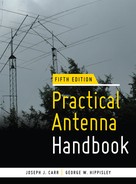
At VHF and above, the ground-plane antenna is a vertical radiator situated immediately above an artificial RF ground consisting of quarter-wavelength radiators or a sheet of highly conductive material such as copper. Most ground-plane antennas are either ¼-wavelength or ![]() -wavelength (although for the latter case impedance matching is needed—see the example later in this chapter).
-wavelength (although for the latter case impedance matching is needed—see the example later in this chapter).
Figure 19.1 shows how to construct an extremely simple ground-plane antenna for 2 m and above. The base of the antenna is a single SO-239 chassis-type coaxial connector. Be sure to use the type that requires four small machine screws to hold it to the chassis, not the single-nut variety.
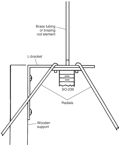
FIGURE 19.1 Construction of VHF ground-plane antenna.
The radiating element is a piece of ![]() -in or 4-mm brass tubing usually obtained at hobby stores that sell model airplanes and modeling supplies. The sizes quoted just happen to fit over the center pin of an SO-239 with only a slight tap from a lightweight hammer. If the inside of the tubing and the connector pin are pretinned with solder, sweat-soldering the joint will make a good electrical connection that is resistant to weathering. Cover the joint with clear lacquer spray for added protection.
-in or 4-mm brass tubing usually obtained at hobby stores that sell model airplanes and modeling supplies. The sizes quoted just happen to fit over the center pin of an SO-239 with only a slight tap from a lightweight hammer. If the inside of the tubing and the connector pin are pretinned with solder, sweat-soldering the joint will make a good electrical connection that is resistant to weathering. Cover the joint with clear lacquer spray for added protection.
Tubing is also used for the radials. Alternatively, solid rods can also be used for this purpose. At least three radials equally spaced around a circle are needed for a proper antenna. (Only two are shown in Fig. 19.1.) For this method of construction, four might be a better number, with one radial attached to each of the four SO-239 mounting holes. Gently flatten one end of the radial with the same small hammer, and drill a small hole in the center of the flattened area. Mount the radial to the SO-239 using hardware of the appropriate size (typically 4-40 screws and nuts for this particular SO-239).
The SO-239 can be attached to a metal L-bracket that is mounted to a length of 2- × 2-in lumber that serves as the mast. While it is easy to fabricate such a bracket from aluminum stock, it is also possible to buy suitable brackets in any well-equipped hardware store.
Coaxial Vertical
The coaxial vertical is a quarter-wavelength vertically polarized antenna that is popular on VHF/UHF. It is really a λ/2 dipole, however, since the exposed quarter-wave center conductor is working against an equal length of exposed shield or braid in line with it, rather than in a ground-plane configuration. The only thing unusual about this antenna is that its method of construction forces the feedline to come away from the antenna inside the braid—an asymmetrical arrangement that has no particular merit and which probably would benefit from the addition of common mode chokes at the bottom of the antenna.
Two varieties of this antenna are usually encountered, depending on how permanent it is supposed to be. In Fig. 19.2A we see the coaxial antenna made with coaxial cable. Although not suitable for long-term installations, it is very useful for short-term, portable, or emergency applications. The length of either the exposed insulation or the exposed shield is found from Eq. (19.1):
FIGURE 19.2A Coaxial vertical based on coaxial cable.
The antenna can be suspended from above with a short piece of string, twine, or fishing line. From a practical point of view, the major problem with this implementation is that the coaxial cable begins to deteriorate after a few rainstorms because the center of the dipole, where the braid and the center conductor go in opposite directions, is exposed to the elements. This effect can be slowed (but not prevented) by sealing the end and the break between the sleeve and the radiator with either silicone RTV or bathtub caulk.
A more weather-resistant implementation is shown in Fig. 19.2B. The sleeve is a piece of copper or brass tubing (pipe) about 1 in in diameter. An end cap is fitted over the end and sweat-soldered into place to prevent the weather from destroying the electrical contact between the two pieces. An SO-239 coaxial connector is mounted on the end cap. The coaxial cable is connected to the SO-239 inside the pipe, which requires making the connection before mounting the end cap.
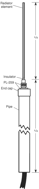
FIGURE 19.2B Tubing coaxial vertical.
The radiator element is a small piece of tubing (or brazing rod) soldered to the center conductor of a PL-259 coaxial connector. An insulator is used to prevent the rod from shorting to the outer shell of the PL-259. (Note: An insulator salvaged from the smaller variety of banana plug can be shaved a small amount with a fine file and made to fit inside the PL-259. It allows enough center clearance for ![]() -in or
-in or ![]() -in brass tubing.)
-in brass tubing.)
Alternatively, the radiator element can be soldered to a banana plug. A standard banana plug nicely fits into the female center conductor of an SO-239.
 -Wavelength 2-Meter Antenna
The ![]() -wavelength antenna (Fig. 19.3) is popular on 2 m for mobile operation because it is easy to construct, and at low elevation angles it provides a small amount of gain relative to the standard λ/4 ground plane. The radiator element is
-wavelength antenna (Fig. 19.3) is popular on 2 m for mobile operation because it is easy to construct, and at low elevation angles it provides a small amount of gain relative to the standard λ/4 ground plane. The radiator element is ![]() -wavelength, so its physical length is found from:
-wavelength, so its physical length is found from:
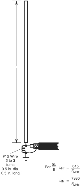
FIGURE 19.3 ![]() -wavelength 2-m antenna.
-wavelength 2-m antenna.
The ![]() -wavelength antenna is not a good match to any of the common forms of coaxial cables. Either a transmission line matching section or an inductor match is normally used. Figure 19.3 shows an inductor match, using a matching coil of two to three turns of #12 wire wound over a ½-in-long ½-in outside diameter (OD) form. The radiator element can be tubing, brazing rod, or a length of heavy piano wire. Alternatively, for low-power systems, it can be a telescoping antenna that is sold as a replacement for portable radios or television sets. These antennas have the advantage of being adjustable to resonance without the need for cutting.
-wavelength antenna is not a good match to any of the common forms of coaxial cables. Either a transmission line matching section or an inductor match is normally used. Figure 19.3 shows an inductor match, using a matching coil of two to three turns of #12 wire wound over a ½-in-long ½-in outside diameter (OD) form. The radiator element can be tubing, brazing rod, or a length of heavy piano wire. Alternatively, for low-power systems, it can be a telescoping antenna that is sold as a replacement for portable radios or television sets. These antennas have the advantage of being adjustable to resonance without the need for cutting.
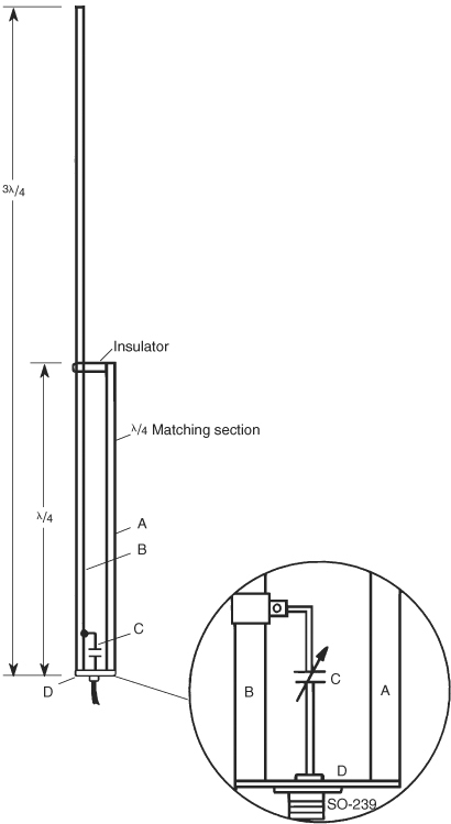
J-Pole Antennas
The J-pole antenna is another popular form of vertical on the VHF bands. It can be used at almost any frequency, although the example shown in Fig. 19.4 is for 2 m. The antenna radiator is ¾-wavelength long, so its length is found from:
![]()
and the quarter-wavelength matching section length from:
![]()
Taken together, the matching section and the radiator form a parallel transmission line with a characteristic impedance that is four times the coaxial cable impedance. If 50-Ω coax is used, and the elements are made from 0.5-in OD pipe, a spacing of 1.5 in will yield an impedance of about 200 Ω. Impedance matching is accomplished by a gamma match consisting of a 25-pF variable capacitor, connected by a clamp to the radiator and tapped about 6 in (experiment with placement) above the base.
Collinear Vertical
Gain in antennas is obtained by “stealing” power from some directions and adding it to other directions. While many of the vertically polarized HF directive antennas we examined in previous chapters have taken energy from one or more azimuthal headings and used it to augment the power radiated in the “forward” direction, it is also possible to obtain gain over a limited range of elevation angles in all compass directions by utilizing energy that might have otherwise gone into elevation angles of little use to us. In this manner it is possible to have a vertical antenna that exhibits gain—at least for certain elevation angles—around the entire 360-degree range of azimuths.
Figure 19.5 is an example of just such an antenna. Through the use of collinear elements for the two sides of a vertical dipole, it develops gain at low elevation angles in an omnidirectional pattern. Each array consists of a quarter-wavelength section A and a half-wavelength section C separated by a phase reversing stub B. (The total length of the stub—out on one side and back on the other—is a half-wavelength, but if made from open-wire line, only a λ/4 line is required. The phase reversal stub adds a 180-degree phase shift between the inner λ/4 section and the outer λ/2 section. Because either outboard half-wavelength section is λ/2 or 180 degrees above or below the center half-wave section, the in-phase currents in the sections cancel in the vertical direction. In any horizontal direction, however, the current in each outer section is in phase with that of its respective inner section, and the antenna exhibits about 3 dB gain at low elevation angles over a conventional λ/2 vertical dipole or λ/4 ground-plane vertical. Note that the phase reversal stub, even if made out of open-wire line, is not being operated as a transmission line and the usual length correction for velocity factor is not applied.

FIGURE 19.5 Vertical collinear antenna.
As is the case with an ordinary dipole, the feedpoint is at the midpoint of the array (i.e., between the A sections). Unlike an ordinary dipole, the free-space feedpoint impedance is around 280 Ω resistive at 146 MHz—a reasonably good match to a 4:1 balun transformer (see Fig. 19.6), especially if fed with 72-Ω coaxial cable. Alternatively, 300-Ω twin-lead can be connected directly to the two sides of the dipole center. If the transmitter lacks the balanced output needed to feed twin-lead, use an appropriate balun at the input end of the twin-lead (i.e., right at the transmitter). For proper performance, make sure the feedline is kept at right angles to the dipole axis near the dipole.
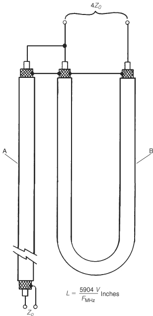
FIGURE 19.6 Coaxial 4:1 balun transformer.
Grounds for Ground-Plane Verticals
With the exception of the sleeve antenna and the collinear dipole, all the preceding verticals are monopoles—in effect, one side of a dipole. All will be poor performers if a good return path simulating the other half of the dipole is not provided. When the base of these antennas is elevated more than a small fraction of a wavelength above ground, an artificial ground plane is an absolute necessity. The simplest way to provide this is with three or four radials cut to λ/4 at the design frequency of the vertical and spaced equally around the compass (120 or 90 degrees apart, respectively). The radials should slope down from the base at about a 45-degree angle. Some experimentation with their exact length and slope may be in order. In contrast to radials laid directly on the earth’s surface, elevated radials are resonant elements, and their length will have a strong effect on both the SWR and the radiation efficiency of the vertical.
Yagi Antennas
The Yagi beam antenna is a highly directional gain antenna and is used in both HF and VHF/UHF systems. The antenna can be easier to build at VHF/UHF than at HF. The basic Yagi was covered in Chap. 12, so we will only show examples of practical VHF devices.
Six-Meter Yagi
A four-element Yagi for 6 m is shown in Fig. 19.7. The reflector and directors can be mounted directly to a metallic boom, but the choice of driven element and its feed system require that the driven element be insulated from the boom.

FIGURE 19.7 Six-meter beam antenna.
The driven element shown in Fig. 19.7 is a folded dipole; because both conductors are the same diameter, it provides a 4:1 step-up in feedpoint impedance relative to a conventional dipole that is largely independent of the ratio of conductor spacing to conductor diameter. Use of a folded dipole for the driven element is common practice at VHF because it tends to broaden the SWR bandwidth of the antenna’s input impedance and because the native feedpoint impedance of Yagis is often very low. For this construction project, two ¾-inch aluminum tubes, spaced 6.5 in apart, were used.
The antenna can be directly fed with balanced 300-Ω line or from 50-Ω or 75-Ω coax through a 4:1 balun. If broadbanding is not important, the folded dipole of the driven element can be replaced with a conventional dipole and the antenna fed directly from a 52- or 75-Ω feedline.
Two-Meter Yagi
Figure 19.8 shows the construction details for a six-element 2-m Yagi beam antenna. This antenna is built using a 2- × 2-in wooden boom and elements made of either brass or copper rod. Threaded brass rod simplifies assembly, but is not strictly necessary. The job of securing the elements (other than the driven element) is easier with threaded rod because it allows securing of each parasitic element with a pair of hex nuts, one on either side of the 2- × 2-in boom. Unthreaded elements can be secured with RTV to seal a press-fit. Alternatively, secure the rods with tie wires (see inset to Fig. 19.8): drill a hole through the 2 × 2 to admit the rod or tubing, secure the element by wrapping a tie wire around the rod on either side of the 2 × 2, and solder it in place. Use #14 to #10 solid bare or tinned wire for the tie wires.

FIGURE 19.8 Two-meter vertical beam.
Mount the mast of the antenna to the boom with an appropriate boom-mast bracket or clamp. One alternative is to use an end-flange clamp, such as is sometimes used to support pole lamps and the like. The mast should be attached to the boom at the center of gravity, also known as the balance point. If you try to balance the antenna on one hand unsupported, there is one (and only one) point at which it is balanced (and won’t tilt end down). Attach the mast hardware at, or near, this point in order to prevent normal gravitational torques from tearing the mounting apart.
The antenna is fed with coaxial cable at the center of the driven element. Often, either a matching section of coax or a gamma match will be needed because the usual effect of parasitic elements on a Yagi’s feedpoint impedance is to make it too low to be a good direct match to standard coaxial cable impedances.
Halo Antennas
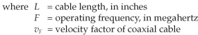
One of the more “saintly” antennas used on the VHF boards is the halo (Fig. 19.9), formed by bending a half-wavelength dipole into a circle. The ends of the dipole are connected to the two plates of a capacitor. In some cases, a transmitting-type mica “button” capacitor is used, but more commonly the VHF halo capacitor consists of two 3-in disks separated by air or plastic dielectric. In some implementations of the halo, the spacing of the disks is adjustable via a threaded screw. While air is a good (and perhaps better) dielectric, the use of a plastic spacer provides mechanical rigidity to help stabilize the exact spacing and, hence, the value of the capacitor.

Quad Beam Antennas
The quad antenna was introduced in Chap. 13. Although much of the discussion there revolved around implementations for HF, it has, nonetheless, also emerged as a very good VHF/UHF antenna. It should go without saying that the antenna is a lot easier to construct at VHF/UHF frequencies than it is at HF frequencies!
Figure 19.10 depicts only one of several methods for building a quad for VHF or UHF. The radiator element can be any of several materials, including heavy solid wire (#8 to #12), tubing, or metal rods. The overall lengths of the elements are given by:

FIGURE 19.10 Quad loop construction on VHF.
![]()
Reflector:
![]()
Director:
![]()
Thanks to this antenna’s lightweight construction, there are several alternatives for making the supports for the elements. In Fig. 19.10, detail A, the spreaders are made from either 1-in furring strips, trim strips, or (above 2 m) even wooden paint-stirring sticks. The sticks are cut to length and then half-notched in the center (Fig. 19.10, detail B). The two spreaders for each element are joined together at right angles and glued (Fig. 19.10, detail C). The spreaders can be fastened to the wooden boom at points S in detail C. Follow the usual rules regarding element spacing (0.15 to 0.31 wavelength). See the information on quad antennas in Chap. 13 for further details. Quads have been successfully employed on all amateur bands up to 1296 MHz.
One commercial variant of the VHF quad is the Quagi—a Yagi that employs a quad driven element.
VHF/UHF Scanner Band Antennas
The hobby of shortwave listening has always had a subset of adherents who listen exclusively to the VHF/UHF bands. Today, scanners are increasingly found in homes but the objective is not shortwave listening (SWLing)—it’s a desire to learn what’s going on in the community by monitoring the police and fire department frequencies.
A few people apply an unusually practical element to their VHF/UHF listening. At least one person known to the author routinely tunes in the local taxicab company’s frequency as soon as she orders a cab. She then listens for her own address and knows from that approximately when to expect her cab!
“Scanner-Vision” Antennas
The antennas used by scanner listeners are widely varied and (in some cases) overpriced. Although it is arguable whether a total-coverage VHF/UHF antenna is worth the money, there are other possibilities that should be considered.
First, don’t overlook the use of television antennas for scanner monitoring! The television bands (about 80 channels from 54 MHz to around 800 MHz) encompass most of the commonly used scanner frequencies. Although antenna performance is not optimized for the scanner frequencies, it is also not terrible on those frequencies. If you already have an “all channel” TV antenna installed, then it is a simple matter to connect the antenna to the scanner receiver with a 2:1 splitter and (possibly) a 4:1 balun transformer that accepts 300 Ω in and produces 75 Ω out. These transformers are readily available at RadioShack and anywhere that TV and video accessories are sold.
The directional characteristic of the TV antenna can be boon or bane to the scanner user. If the antenna has a rotator, then there is no problem. Just rotate the antenna to the direction of interest (unless someone else in the family happens to be watching TV at the time!). But much of the time it won’t even be necessary to rotate the TV/FM antenna—partly because no antenna completely rejects signals arriving from off the sides or the back, and partly because most of the local scanner repeaters will be quite strong.
An excellent alternative to hijacking the family’s primary TV antenna is to locate an indoor set-top TV antenna at a garage sale or flea market (or maybe your own attic). Some of these have a simple phasing circuit built in with a front panel knob that allows the user to move the peak of the antenna pattern around some. With the possible addition of a wideband TV antenna preamplifier (available at RadioShack, among other places), such a setup may be perfectly adequate for scanner monitoring.
Scanner Skyhooks
Some popular scanners even cover much of the HF spectrum. For true SWLing on those bands, a random-length wire antenna ought to turn in decent performance, and it may even be able to do double duty as a VHF/UHF longwire antenna. Typically, this antenna is simply a 30- to 150-ft length of #14 wire attached to a distant support.
Additional gain, about +3 dB, can be achieved by stacking VHF/UHF antennas together. Figure 19.11 shows a typical arrangement in which two half-wavelength dipole antennas are connected together through a quarter-wavelength harness of RG-59/U coaxial cable. This harness is physically shorter than an electrical quarter-wavelength by the velocity factor of the coaxial cable:
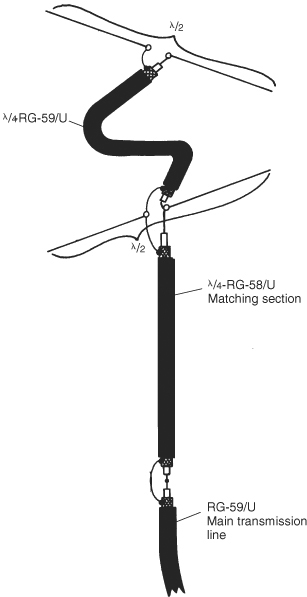
FIGURE 19.11 Stacking VHF antennas.
![]()
![]()
The antennas can be oriented in the same direction to increase gain, or orthogonally (as shown in Fig. 19.11) to obtain a more omnidirectional cloverleaf pattern.
Because the impedance of two identical dipoles, fed in parallel, is one-half that of a single dipole, it is necessary to have an impedance-matching section made of RG-58/U coaxial cable. This cable is then fed with RG-59/U coax from the receiver.
There is nothing magical about scanner antennas that is significantly different from other VHF/UHF antennas except, perhaps, the need to cover multiple frequency ranges. Although the designs might be optimized for VHF or UHF, these antennas are basically the same as others shown in this book. As a matter of fact, almost any antennas, from any chapter, can be used over at least part of the scanner spectrum.
VHF/UHF Antenna Impedance Matching
VHF/UHF antennas are no different from their HF brethren in their need for impedance matching to the feedline. However, some methods (coax baluns, delta match, etc.) are easier at the higher frequencies, while others become difficult or impossible. An example of the latter case is the tuned LC impedance-matching network. At 6 m, and even to some extent at 2 m, lumped-component LC networks can be used. But at 2 m and above, other methods are often easier to implement. For example, we can replace the LC tuner with stripline tank circuits.
The balun transformer provides an impedance transformation between balanced and un balanced circuit configurations. Although both 1:1 and 4:1 impedance ratios are possible, the 4:1 ratio is most commonly used for VHF/UHF antenna work. At lower frequencies it is easy to build broadband transformer baluns, but these become more of a problem at VHF and above.
Figure 19.6 is a 4:1 impedance ratio coaxial balun often used on VHF/UHF frequencies. Two sections of identical coaxial cable are needed. One section (A) can be any convenient length needed to reach from the antenna to the transmitter. Its characteristic impedance is Z0. The other section (B) is cut to be a half-wavelength long at the center of the frequency range of interest. The physical length is found from
![]()
The velocity factors of common coaxial cables are shown in Table 19.1.

TABLE 19.1 Coaxial Cable Velocity Factors
Hard line velocity factors typically lie in the 0.8 to 0.9 range, but it is wise to check the manufacturer’s specifications for the exact number. Alternatively, a better approach for either coaxial cable or hard line is to measure the velocity factor of the specific piece of cable you intend to use. See Chap. 27 (“Instruments for Testing and Troubleshooting”) for more information.
Example 19.1 Calculate the physical length required of a 146-MHz 4:1 balun made of polyethylene foam coaxial cable.
Solution

One approach to neatly joining the coaxial cables is shown in Fig. 19.12. In this example, three SO-239 coaxial receptacles are mounted on a metal plate. This arrangement has the effect of shorting together the shields of the three ends of coaxial cable while the center conductors are connected in the manner shown. This method is sometimes provided as part of a commercial antenna; the author’s commercial 6-m Yagi has just such a bracket on it, the only difference being the use of BNC connectors.

FIGURE 19.12 Practical implementation of 4:1 balun using connectors.
Because the balun of Figs. 19.6 and 19.12 is mounted at the antenna feedpoint and, hence, is almost always located outdoors, special care must be taken to weatherproof the ends of the transmission line—especially the long run back to the transmitter.
The delta match gets its name from the fact that the physical layout of the matching network used when tapping out on the two sides of a driven element or dipole a distance corresponding to the transmission line impedance has the shape of the Greek letter delta. Figure 19.13A shows the basic delta match scheme. The delta match connections to the driven element are made symmetrically on both sides of center, and can be made from brass, copper, or aluminum tubing, or a bronze brazing rod bolted to the main radiator element.

FIGURE 19.13A Delta feed matching system.
The width (A) of the delta match is given by
![]()
while the length (B) of the matching section is
![]()
The transmission line feeding the delta match is balanced line, such as parallel transmission line or twin-lead. The exact impedance is not terribly critical because the dimensions (especially A) can be adjusted for a good match. Although 450-Ω line is commonly used, 300-Ω or 600-Ω lines are equally good alternatives. Figure 19.13B shows a method for using coaxial cable or hard line with the delta match. The 50- or 75-Ω coax or hardline impedance is transformed up to the delta match impedance with a 4:1 balun transformer such as the one in Fig. 19.6.
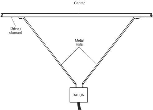
FIGURE 19.13B Practical VHF delta match.
A stub-matching system is shown in Fig. 19.14. The exact impedance of the line is not very critical and is found from
![]()
where S is the space between the two sides of the line and d is the diameter of each conductor.
The matching stub section is made from metal elements such as tubing, wire, or rods, since all three are practical at VHF/UHF frequencies. For a ![]() -in rod, the spacing is approximately 2.56 in to make a 450-Ω transmission line. A sliding short circuit sets the electrical length of the half-wave stub. The stub is tapped at a distance from the antenna feedpoint that matches the impedance of the transmission line. In the example shown, the transmission line is coaxial cable, so a 4:1 balun transformer is used between the stub and the transmission line. The two adjustments to make in this system are: (1) the distance of the short from the feedpoint and (2) the distance of the transmission line tap point from the feedpoint. The two are alternately adjusted for minimum VSWR.
-in rod, the spacing is approximately 2.56 in to make a 450-Ω transmission line. A sliding short circuit sets the electrical length of the half-wave stub. The stub is tapped at a distance from the antenna feedpoint that matches the impedance of the transmission line. In the example shown, the transmission line is coaxial cable, so a 4:1 balun transformer is used between the stub and the transmission line. The two adjustments to make in this system are: (1) the distance of the short from the feedpoint and (2) the distance of the transmission line tap point from the feedpoint. The two are alternately adjusted for minimum VSWR.
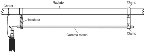
The gamma match is basically a half-delta match and operates according to similar principles (Fig. 19.15). The shield (outer conductor) of the coaxial cable is connected to the exact center of the driven element. The center conductor of the coaxial cable series feeds the gamma element through a variable capacitor.