CHAPTER 23
Radio Direction-Finding (RDF) Antennas

Radio direction finding is the art and practice of using antenna directivity to pinpoint either your own location or that of a distant source of RF energy. When the Federal Communications Commission (FCC) or other telecommunications authorities want to locate an illegal station that is transmitting, one of their primary tools is the use of radio direction finders to triangulate the bootleg station’s position. In the same way that the global positioning system (GPS) receiver in your navigation system or smart phone determines where you are located, monitors can determine the location of another station from the intersection of bearing lines obtained at two or more receiving sites. In contrast to the bearing accuracy available from GPS satellites, there is a fair degree of ambiguity in bearings obtained for terrestrial targets—especially on the MF and HF bands—because multiple propagation modes, paths, and anomalies can easily obscure the true bearing of the signal source. As a result, radio direction finders typically use three or more sites. Each receiving site that can find a bearing to the station reduces the overall error.

At one time, aviators and seafarers relied on radio direction finding. It is said that the Japanese air fleet that attacked Pearl Harbor, Hawaii, on December 7, 1941, homed in on a Honolulu AM broadcast station. During the 1950s and early 1960s, AM radio dials in the United States were marked with two little circled triangles at 640 and 1240 kHz. These were CONELRAD frequencies that people were encouraged to tune to in case of a nuclear attack. In each area of the country multiple selected radio stations would occupy a CONELRAD frequency, taking turns transmitting in a carefully orchestrated (and secret) sequence. At the same time, all radio stations except assigned CONELRAD stations would have to cease transmitting. Thus, local broadcast news and information services could be maintained at the same time the enemy was being prevented from using any AM broadcast signals for RDF because no one CONELRAD station was on the air long enough to allow a fix.

Radio direction-finding equipment utilizing the AM broadcast band (BCB) looks much like Fig. 23.1. A receiver with an S-meter to measure signal strength is equipped with a rotatable ferrite loopstick antenna to form the RDF unit. A 360-degree scale around the perimeter of the antenna base can be rotated to line up with true north so that compass bearing can be read off directly.

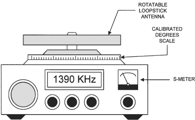
FIGURE 23.1 Radio direction-finding (RDF) receiver with loopstick antenna.

Loopstick antennas exhibit a figure eight reception pattern (Fig. 23.2A) with the maxima (lobes) parallel to the loopstick rod and the minima (nulls) off the ends. When the antenna is broadside to the signal source, received signal strength is maximum. Unfortunately, the maxima are so broad that it is virtually impossible to find the true point on the compass dial where the signal peaks. Fortunately, the minima are very sharp, and a good fix on the source can be obtained by nulling the signal, instead of peaking it. The null is found by rotating the antenna until the audio disappears or the S-meter dips to its minimum observed value (Fig. 23.2B).

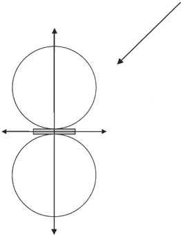
FIGURE 23.2A Pattern of loopstick antenna: random orientation of source.

FIGURE 23.2B Pattern of loopstick antenna: nulling the source.

The loopstick is a really neat way to do RDF—except for one little problem: The darn thing is bidirectional! There are two minima because the antenna pattern is symmetrical about the antenna’s axis. You will get exactly the same response from aiming either end of the stick in the direction of the station. As a result, the unassisted loopstick can only show you a line along which the radio station is located but can’t tell you which half of the line to focus on. Sometimes this doesn’t matter; if you know the station is in a certain city and that you are generally south of the city, and can distinguish the general direction from other clues, then the half of the null line that is closer to the north will provide the answer.

One solution to the ambiguity problem is to add a sense antenna to the loopstick (Fig. 23.3). The sense antenna is an omnidirectional vertical whip, and its signal is combined with that of the loopstick in an RC phasing circuit. When signals from the two antennas have roughly equal amplitudes, the resultant pattern will resemble Fig. 23.4. This pattern is called a cardioid because of its heart shape. Because it has only one null, it resolves the ambiguity of the loopstick pattern.

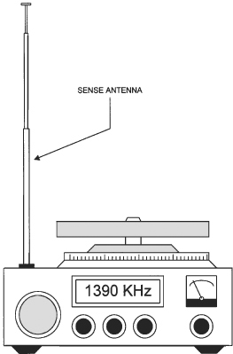
FIGURE 23.3 Addition of sense antenna overcomes directional ambiguity of the loopstick.

FIGURE 23.4 Cardioid pattern of sense-plus-loopstick antennas.

Note, however, that a single RDF receiver can provide only bearing information. Receivers at two or more sites, widely separated (relative to bearing angle of the target), are necessary to also obtain distance information and pinpoint the location of the target.

Field Improvisation

Suppose you are out in the woods trekking around the habitat of lions, tigers, and bears (plus a rattlesnake or two for good measure). Normally you find your way with a compass, a U.S. Geological Survey 7.5-min topological map, and a GPS receiver. Those little GPS marvels can usually give you excellent latitude and longitude indication when you can see sky above you, but often fail to deliver reliable position information in woodlands and dense forests. In such terrain, the answer to your direction-finding problem might be the little portable AM BCB radio (Fig. 23.5) that you brought along for company.

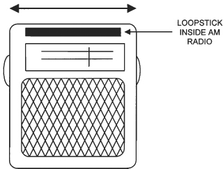
FIGURE 23.5 AM portable radio. Dark bar represents position and direction of internal loopstick.

Open the back of the radio and find the loopstick antenna, because you will need to know its orientation. In the radio shown in Fig. 23.5 the loopstick lies across the top of the radio, from left to right, but in other radios it is vertical, from top to bottom. Once you know its position, you can tune in a known AM station and orient the radio until you find a null. Next, point your compass in the same direction to obtain the numerical bearing (0–360°) of the signal. If you know the approximate location of the broadcast station, subtract the bearing you determined from 180 degrees (or vice versa, depending on which method gives you a positive value equal to 360 or less) and draw a line on the topo map at that angle, originating at the known AM broadcast station. Of course, it’s still a bidirectional indication, so all you know is the line along which you are lost.

Now tune in a different station in a different city (or one at least far enough from the first station to make a difference) and take another reading. Again subtract (or add) 180 degrees to obtain a positive number between 0 and 360. Draw a line at this bearing originating from the second broadcast station location. These two lines should intersect at your approximate location. If you know the locations of additional broadcast stations, take a third, fourth, and fifth reading and you will generally be able to pinpoint your location pretty tightly. If you were smart enough to plan ahead, you will have selected candidate stations in advance and located the latitude and longitude coordinates of each. Alternatively, you would have brought topo maps premarked with their locations as well as where you plan to hike, and from those maps you can find the latitudes and longitudes of the distant stations.

With the appropriate receiver, the same technique works as well with FM stations, although it’s important not to let multipath propagation modes (see Chap. 4) confuse you.

Loop Antennas for RDF

Conventional wire loop antennas (Fig. 23.6) are also used for radio direction finding. In fact, in some cases the regular loop is preferred over the loopstick. The regular loop antenna may be square (as shown), circular, or any other equi-sided “n-gon” (e.g., hexagon), although the square is generally easiest to build. Only a few turns are needed to accumulate adequate inductance for resonating in the AM broadcast band with a standard 365-pF “broadcast” variable capacitor. For a square loop 24 in on a side (dimension A in Fig. 23.6), about 10 turns of wire spaced over a 1-in width (B in Fig. 23.6) should be sufficient. For portable direction finding, a small loop can be mounted to the top of a rigid support mast such as a length of 2- × 4-in lumber, as shown in Fig. 23.7. The important design constraints are that the loop is high enough to have some separation from your vehicle (if you need to stand close to it in order for the feedline to reach the receiver) and that the loop is never so high that it can touch the lowest power lines in the vicinity.

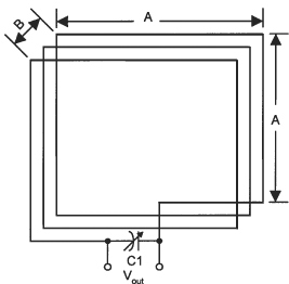
FIGURE 23.6 Wire loop antenna.

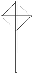
FIGURE 23.7 Simple portable RDF loop antenna.

Be aware that the small loop antenna has a figure eight pattern like the loopstick, but the maxima and minima are oriented 90 degrees from those of the loopstick. In the regular loop the nulls are perpendicular to the plane of the loop, while the maxima are off the sides. Thus, in Fig. 23.6 the nulls are in and out of the page, while the main lobes are left and right (or top and bottom).

Sense Antenna Circuit

Figure 23.8 shows a method for summing together the signals from an RDF antenna (such as a loop) and a sense antenna. The two terminals of the loop are connected to the primary winding of an RF transformer. This primary (L_1A) is centertapped and the centertap is grounded. The secondary of the transformer (L_1B) is resonated by a variable capacitor C₁. The dots on the transformer coils indicate the 90-degree phase points.

FIGURE 23.8 Sense circuit for a loop/sense antenna RDF.

The top of L_1B is connected to both the sense circuit and the receiver antenna input. Potentiometer R₁ is a phasing control. The value of this pot is usually 10 to 100 kΩ, with 25 kΩ common. Switch S₁ is used to disconnect the sense antenna from the circuit. Because the nulls of the loop or loopstick are typically a lot deeper than the null on the cardioid pattern, the null is first located with the switch open. If the receiver S-meter reading drops when the switch is closed, the correct null has been selected. If not, reverse the direction of the antenna and repeat the process.

RDF at VHF and UHF

It should be apparent from the preceding paragraphs that obtaining an easily portable antenna with a unidirectional pattern at HF requires some mechanical and electronic complexities. At VHF and above, such patterns are far easier to attain. Even a four-element 6-m Yagi is reasonably easy to manipulate by hand, and the task gets simpler as one goes higher in frequency. At even higher frequencies, the antenna of choice is the parabolic reflector.

Perhaps a more difficult task at VHF and above is finding a way to get signal strength information from the receiver being used. In today’s marketplace, very few VHF/UHF FM mobile rigs include any visual metering, even when the AM aircraft band is present. A rare rig may have a dc voltage proportional to received signal level available on the rear panel, but the most likely transceivers to have S-meters (or their modern equivalent, the LED “bar” meters) are the relatively expensive “multimode” rigs intended primarily for base station use.

Fox Hunting

An activity popular with ham radio operators for many decades is fox hunting. A fiendishly clever ham (the “fox”) would hide with a mobile or portable transmitter (usually on either 10 or 75 m). The “hunters” would then RDF the fox’s brief transmissions and try to locate the transmitter. If you were first to locate the antenna, you won—and got to be the fox the following month!

Today, fox hunting is as likely to be held on VHF and UHF as on the lower frequencies. Because the propagation modes can be so different around a geographic region, both types provide many lessons.

Tracking Down Electrical Noise

A practical use for fox hunting skills is tracking down sources of electrical noise that can mask weak signals. Most electrical noise comes from close by: every electrical appliance that plugs into the wall (and even a few that don’t!), every wall adapter, every computer or fax machine or wireless modem, every power line and power pole, every high-efficiency heating or cooling system, every on-demand hot water heater, every electric blanket, every touch lamp, and every streetlight or yard light is a suspect until proven “innocent”. In most cases, a good technique is to start your “fox hunting” activities on the frequencies where you first noticed the noise and then gradually move upward in frequency as you get closer to the source. There are at least three reasons for that:

• Noise energy in the VHF and UHF ranges is not likely to travel via as many ambiguous propagation paths that can lead to contradictory results.

• Noise energy in the VHF and UHF ranges from most unintentional radiators is much weaker than at the lower frequencies; if you can hear it at all at VHF and UHF, you’re probably very close to the source.

• It’s far, far easier to hold and rotate a high-gain, sharp beam VHF or UHF antenna by hand than it is to get the same directivity on HF!

Here are some additional hints for locating that stubborn noise that’s wiping out your weak-signal reception on the HF bands:

• Power line and power pole noises are particularly difficult because the noise can propagate for miles along the lines and go through many maxima and minimum before tapering off. Don’t let one of those maxima cause you to jump to conclusions.

• Do your initial “hunting” quickly and easily while mobile by tuning the AM broadcast radio in your car to an unused frequency near the top of the broadcast band (somewhere in the 1600- to 1700-kHz range). The author found an offending municipal streetlight near his home in this manner.

• Keep your portable receiver in AM mode if at all possible. When it’s time to switch to VHF antennas, amateur 2-m FM handhelds or mobile rigs that include coverage of the AM aircraft band between 108 and 130 MHz are especially useful for zeroing in on a specific power pole or building.

• Keep a log of dates, times, day/night status, and weather conditions each time you observe the noise. Some noises are the result of arcing when insulating surfaces get wet; others are the exact opposite. Some noises result from outdoor lighting powered by day/night sensors, and so on.

• To determine if the noise source is in your own home, turn off your house power at the main breaker box at a time when the noise is evident in your receiver. Continue to run your equipment on a 12-V car battery or an uninterruptible power supply (UPS). However, don’t forget that UPSs and other battery-operated devices may continue to run for hours on their own and are fully capable of creating RFI long after primary power has been removed.

• Be careful, courteous, and circumspect when checking out noises potentially emanating from a neighbor’s house; otherwise you may end up in front of the local judge, charged with being a “peeping Tom”!

CAUTION Never, under any circumstances, “body-slam” a power pole or hit it with a sledgehammer or your vehicle’s bumper to see if the offending noise is coming from it! Besides being highly illegal, this could be sure death if the trouble is, in fact, with any of the equipment on the pole. If you have reason to suspect a specific section of utility wiring, go back home and report your concern directly to your utility.

The usual lack of an S-meter on mobile or portable VHF/UHF receivers is as much a problem for tracking down noise sources as it is for RDFing on distant stations. However, one possible work-around while listening to the AM aircraft band— if the background noise environment is favorable—is to employ the audio noise output of the speaker in a mobile VHF/UHF rig in conjunction with an audio signal level monitor app for a smart phone. Examples of apps currently available for the Apple iPhone include Sound Level (and Sound Level Pro). As with the S-meter approach, two operators are typically required—one to maneuver the antenna and another to watch the meter and call out “Warmer!” or “Colder!” as the signal level goes up or down.

Shortwave and AM BCB “Skip” RDF

Radio direction finding is most accurate over relatively short distances. If you have the choice, it’s better to use the ground wave (which is what you use during daylight hours for nearly all AM BCB stations). Skip rolls in on the AM BCB after local sundown, so you can hear all manner of stations up and down the dial. However, with a little practice, you can even RDF distant stations.

Unfortunately, there are some practical difficulties associated with skip RDFing. When we look at propagation drawings of skip in textbooks we usually see what’s happening in a single plane at a time. Typically, a single imagined “pencil beam” radio signal is shown traveling at some angle up the ionosphere, where it is “reflected” (actually, it’s a refraction phenomenon but looks like reflection to an observer on the surface) back to earth. We can tell from the drawing that the angle of incidence equals the angle of reflection, just like they told us in high school science classes. Unfortunately, the real world is not so neat and crisp.

In the real world the skywave signal we hear is an amalgam of many such “pencil beams”, coming in from a near-infinite number of directions and elevation angles. The strongest component of such a signal aggregate is always the path that has the least total loss from start to end, but for skip distances that path is always shifting because the ionosphere that makes skip reception possible is a continuously shifting medium. A radio wave refracting through the ionosphere must feel like you and I do when taking a ride through the house of warped mirrors at an amusement park. It’s entirely possible, therefore, that at any given instant the preferred path to your antenna for a signal source located to the northwest of you might be a so-called skew path, coming in from as far around the compass rose as the southwest!

Terrestrial reflections also cause problems, especially when RDFing a station in the high end of the HF band or the VHF/UHF bands. Radio waves will reflect from geological features such as mountains and from man-made structures (e.g., buildings). If the reflection is strong enough, it might appear to be the real signal and cause a severe error in RDFing.

Bottom line: Be wary of RDF results on HF when the “skip is in”. Similarly, don’t let the canyons of New York City or the mountains of upstate fool you on VHF and UHF.

Adcock Antennas

The Adcock antenna (Fig. 23.9) has been around since 1919, when it was patented by British Royal Engineer and Lieutenant Frank Adcock as a way of overcoming the tendency of RDF loops to lose directional accuracy at nighttime. Adcock surmised that the horizontally polarized component of incoming skywave signals induced loop output voltages indicating certain spurious directions when the output voltage due to the vertically polarized ground wave was near zero. To minimize this error, Adcock designed a number of different configurations based on the use of vertical elements, both monopole and dipole.

FIGURE 23.9 Adcock array RDF antenna.

The Adcock antenna shown here once found use in the United States by the FCC at their old monitoring sites. It consists of two center-fed, nonresonant (but identical) vertical radiators. Each side of each element is at least 0.1λ long, but need not be resonant (which means the antenna can be used over a wide band). The elements are spaced from 0.1λ to 0.75λ, although the example shown here is spaced 0.125λ. Spacing is ultimately limited by the need to avoid distorting the circular (omnidirectional) pattern of each element in the pair, so a given dipole configuration is suitable over only a 3- or 4-to-1 frequency range. Pickup of horizontally polarized signals on the feedline to each element is minimized through the use of balancing or shielding techniques.

Other Adcock arrays are designed around two pairs of vertical dipoles or monopoles. All Adcock antennas are vertically polarized and respond only to vertically polarized waves, so they have earned an excellent reputation as being superior to loops for precise high-frequency shortwave RDFing.

A typical pattern for an Adcock antenna is shown in Fig. 23.10. This pattern was generated by modeling the array using the NecWin Basic for Windows program (Chap. 25). The example antenna is a 10-MHz (30-m band) Adcock that uses 1.455-m elements (total 2.91 m on each side), spaced 4 m apart. The pattern is a traditional figure eight with deep nulls at 0 degrees and 180 degrees. The antenna can be rotated to find a null in the same manner as a loop.

FIGURE 23.10 Adcock pattern.

Watson-Watt Adcock Array

Figure 23.11 shows the Watson-Watt Adcock RDF array, consisting of two Adcock pairs arranged orthogonally to each other. It is common practice to align one Adcock with an east-west line and the other with north-south. These are fed to identical receivers that are controlled by a common local oscillator (LO). The outputs of the receivers are balanced and are used to drive the vertical and horizontal plates of a cathode-ray oscilloscope (CRO). Figure 23.12 shows the patterns that result when signals of various phases arrive at the Watson-Watt array. The patterns of Figs. 23.12A and 23.12B are from signals 180 degrees out of phase, while the pattern of Fig. 23.12C is the result of a 90-degree phase difference.

FIGURE 23.11 Watson-Watt Adcock array.

FIGURE 23.12 Patterns for different signals on the Watson-Watt array.

Doppler RDF Antennas

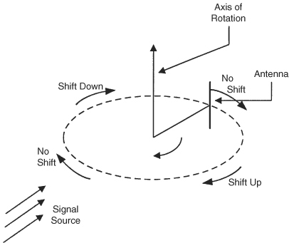
Figure 23.13 shows the basic concept of an RDF antenna based on the Doppler effect, which was discovered in the nineteenth century. A practical example of the Doppler effect is seen when an ambulance with wailing siren first approaches a stationary observer, then passes beyond. The pitch of the siren heard by the motionless observer is initially at its highest (and higher than the pitch heard at the source by the driver of the ambulance). It continuously drops as the source approaches and then passes by. Although useful, the acoustic analogy is not perfect, since the Doppler mechanism for EM waves in a vacuum is a little bit different than that for the subsonic acoustic waves of the ambulance.

FIGURE 23.13 Doppler antenna.

In a radio system, when distance between a receiving antenna and a signal source is changing, a Doppler shift in the received signal frequency is detected; the amount of shift is proportional to the differential radial velocity between the two. (No Doppler shift occurs as a result of any change in motion at right angles to the line connecting the source and the receiver.) Thus, when a hobbyist listens to the telemetry signals from a passing satellite or the international Morse code (CW) of a radio amateur making contacts through an AMSAT repeater satellite (visit www.amsat.org), the received frequency continuously slides lower as the satellite comes into radio “view”, passes nearby, and finally disappears until its next orbit. At the point of the satellite’s closest approach to the receiving station (whether directly overhead or off to the side), the received frequency equals the actual transmitted frequency because neither antenna has any radial velocity relative to the other for that brief moment. Before then, the received frequency is higher; afterward, it is lower.

The Doppler RDF antenna of Fig. 23.13 rotates at a constant angular velocity. The signal wavefront approaches from a single direction (the lower left corner of the illustration in this example), so there will be a predictable Doppler shift at any point on the circular path of the antenna. The magnitude of the frequency shift is maximum when the antenna is moving directly toward the source or away from it—i.e., when it is on either side of the figure. When the antenna is closest to the source or farthest from it, there is very little Doppler shift. The maximum shift at the two sides can be found to be

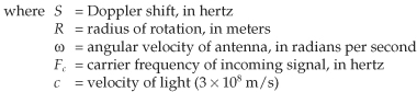
In theory this antenna works nicely, but in practice there are problems, one of which is getting a Doppler shift large enough to easily measure. Unfortunately, the mechanical rotational speed required of the antenna is very high—too high for practical use. However, the effect can be simulated by sequentially (i.e., electronically) scanning a number of antennas arranged in a circle. The result is a piecewise approximation of the effect seen when the antenna is rotated at high speed. Byonics (www.byonics.com) offers a kit by Daniel F. Welch, W6DFW, that incorporates the N0GSG Doppler system with digital signal processing (DSP) originally described in the November 2002 issue of QST. In this system, four verticals are electronically switched at high speed to create the Doppler shift that allows pinpointing of the source to a 22.5 percent segment of the compass rose. The user is responsible for constructing the four verticals. Googling the words “Doppler RDF antenna” will provide numerous hits on the topic.

Wullenweber Array

One of the problems associated with small RDF antennas is that relatively large distortions of their pattern result from even small anomalies because they have such a small aperture. If you build a wide-aperture direction finder (WADF), however, you can average the signals from a large number of antenna elements distributed over a large- circumference circle. The Wullenweber array (Fig. 23.14) is such an antenna. It consists of a circle of many vertical elements. For HF the circle can be 500 to 2000 ft in diameter!

FIGURE 23.14 Wullenweber RDF array.

A goniometer rotor spins inside the ring to produce an output that will indicate the direction of arrival of the signal as a function of the position of the goniometer. The theoretical resolution of the Wullenweber array is on the order of 0.1 degree, although practical resolutions of less than 3 degrees are commonly seen.

Time Difference of Arrival (TDOA) Array

If two antennas are erected at a distance d apart, arriving signals can be detected by examining the time-of-arrival difference. Figure 23.15A shows a wavefront advancing at an arbitrary angle to the line between two antennas. If the wavefront is parallel to the antenna axis, it will arrive at both antennas at the same time. But if the signal arrives at an angle, it will arrive at one antenna some time before it reaches the second. From the difference in the arrival times at the two antennas we can calculate the arrival angle.

FIGURE 23.15A Time difference of arrival (TDOA) RDF array.

There is an ambiguity in the basic TDOA array in that the combined output will be the same for conjugate angles, i.e. at the same angle on opposite sides of a line bisecting the array. This problem can be resolved by adding the electronic system of Fig. 23.15B. Signals from ANT1 and ANT2 (designated V₁ and V₂, respectively) are detected by separate receivers (RCVR1 and RCVR2) and then threshold detected in order to prevent signal-to-noise problems from interfering with the operation. The outputs of the threshold detectors are used to trigger a sawtooth generator that controls the horizontal sweep on an oscilloscope. The two signals are then delayed, and one is inverted so that the operator can distinguish between their traces on the CRT screen, thus eliminating the ambiguity.

FIGURE 23.15B Block diagram of typical TDOA circuit.

Example: If the antennas in Fig. 23.15A are arrayed east and west, the line perpendicular to the line drawn between them runs north and south. If we designate north as 0 degrees, the signal shown arrives at an angle of 330 degrees, and it will arrive at ANT1 before it arrives at ANT2. A signal arriving from a bearing of 30 degrees will produce the same output signal, even though it arrives at ANT2 before ANT1. All signals of bearing 0 ≤ θ < 180° will arrive at ANT2 first, while all signals 180 ≤ θ < 360° will arrive at ANT1 first. Yet both will produce the same blip on the oscilloscope screen. The solution to discerning which of the two conjugate angles is the true arrival angle is to invert the ANT1 signal. When this is done, the ANT1 signal falls below the baseline on the CRT screen, while the ANT2 signal is above the baseline. By noting the time difference between the pulses and their relative positions, we can determine the bearing of the arriving signal.

Switched-Pattern RDF Antennas

If an advancing wavefront arrives at two identical antennas from a direction perpendicular to the line connecting the antennas, the phase of the wavefront will be the same at both antennas. If signals from the two antennas are “chopped” at an audio rate with a square wave and alternately fed to a simple receiver, the resulting phase modulation will appear as an audio tone at the receiver output. Rotation of the antenna array until the tone is nulled out, which occurs when there is no phase difference between the signals at the two antennas, provides an accurate bidirectional “fix” on the source of the wavefront.

Double-Ducky Direction Finder (DDDF)

Figure 23.16 shows in simplified form a system originally presented to amateur radio operators by David T. Geiser, W5IXM, for use with “rubber ducky” VHF antennas; he called it the double-ducky direction finder (DDDF). Because of the sharpness of the null, Geiser chose to use these short, loaded, and rubber-damped antennas rather than full λ/4 or 5/8λ whips because vibration and wind can cause enough relative motion between elements of an array built with full-length whips to make it difficult to get a clean null in normal outdoor use.

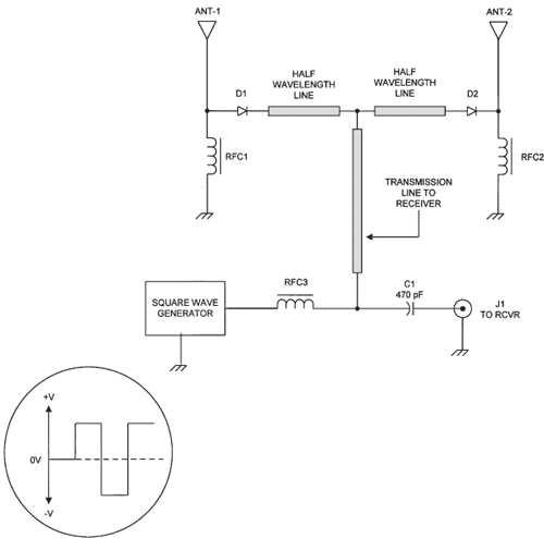
FIGURE 23.16 Double-ducky switched-pattern RDF system.

Spacing of the two antennas is not critical; 0.25λ to 1λ apart over a good ground plane (such as the roof of a car or truck) should work well. As with all vertical monopoles, if no ground plane exists, a sheet metal ground plane should be provided.

In Fig. 23.16 the antennas are fed from a common transmission line to the receiver. In order to keep them electrically the same distance apart, identical half-wavelength sections of transmission line are used to connect the antennas to the shared section of line.

Switching is accomplished by using a bipolar square wave and PIN diodes. The bipolar square wave (see inset to Fig. 23.16) has equal positive and negative peak voltages on opposite halves of the cycle. The PIN diodes (D₁ and D₂) are connected in opposition such that diode D₁ conducts on negative excursions of the square wave and D₂ conducts on positive excursions. In any given half-cycle of the audio frequency square wave, one antenna is connected to the receiver when its diode is conducting and the other diode is back-biased, creating a high impedance between its antenna and the shared line. Thus, the active antenna alternates rapidly between ANT1 and ANT2.

The combined signal from the two antennas is coupled to the receiver through a small-value capacitor (C₁) that blocks the baseband audio frequency square wave from appearing at the receiver input. This allows use of the shared transmission line segment for both the RF signal and the switching signal. An RF choke (RFC₃) is used to keep RF from the antenna from entering the square-wave generator.

The DDDF antenna phase-modulates the incoming signal at the frequency of the square wave, and the resulting tone can be heard in the receiver output. When the signal’s direction of arrival is perpendicular to the line between the two antennas, the phase difference is zero and the audio tone disappears.

The pattern of the DDDF antenna is bidirectional, so the ambiguity problem found with loop antennas exists here, as well. In this system the ambiguity can be resolved by either of two methods:

• Place a reflector λ/4 behind each antenna. This is an attractive solution, but it tends to distort the antenna pattern a little bit.

• Rotate the antenna through 90 degrees (or walk an L-shaped path).

Summary

This chapter has touched on the basics of radio direction finding. Much more depth can be found on the Internet and in newsletters from clubs and others specializing in RDF technology and techniques. RDF can be very useful for locating RF sources, both good and bad; as such, it is an important tool for locating illegal stations or undesired noise sources. RDF is a great way to build club spirit and teach a wide variety of technical concepts through fox-hunting training exercises and group construction projects. It can also be used to determine your own location if you can get bearings on at least two RF sources at known positions. Try it . . . you’ll like it!