
CHAPTER 25
Antenna Modeling Software
One of the significant contributions of computer technology to the field of antennas is the availability of modeling and simulation tools that eliminate most of the drudgery associated with the complex calculations involved in analyzing and optimizing antenna designs. For most readers of this book, the best part of this is the extension of those tools to personal computers at very modest prices and even for free! Today, any individual interested in experimenting with novel antenna configurations can do so, and in the process spend little or nothing on modeling software.
Modeling and simulation are used in a wide variety of applications, including management, science, and engineering. We can now model just about any process, any device, or any circuit that can be described mathematically. The purpose of modeling, at least in engineering, is to validate the design quickly and cheaply on the computer before “bending metal”. Modeling and simulation make it possible to look at alternatives and gauge the effect of a proposed design change before the change is actually implemented. The old “cut and try” method works, to be sure, but it is costly in both time and money—two resources perpetually in short supply. If performance issues and problems can be solved on a computer, then we are time and money ahead of the game.
Nowhere is this more true than in the field of antennas, where each design iteration historically involved lowering the antenna from its support, adjusting its dimensions, reinstalling it many feet up in the air, and conducting a new round of test measurements. Alternatively, towers with sizeable nonconducting work platforms were utilized, and all the physical adjustments and fine-tuning accomplished “up topside”—in situ, as it were. A half-century ago or less, antenna test ranges with these capabilities were found only at government research centers and commercial antenna manufacturers’ facilities.
Under the Hood
Virtually all commonly available antenna modeling software for personal computers is based on a numerical analysis technique known as the “method of moments”, in which each wire or antenna element in the system is broken into many short segments, and the current in each segment is calculated based on the rules of electromagnetism and the boundary conditions seen by each segment. The fields generated by the antenna are determined by summing the contributions of all wire segments throughout model space, varying both azimuth and elevation angle to compute, tabulate, and graphically plot relative field strength compared to an isotropic radiator as a function of angular position from the antenna for a constant RF drive power applied to the antenna feedpoint(s). Ancillary data, including plots of voltage standing wave ratio (VSWR) versus frequency, calculation of feedpoint voltage and current, currents in all wire segments, etc., are also available.
The core for most of the programs in use today was originally developed for the U.S. Navy. Called the Numerical Electromagnetic Computation (NEC) program, it has had a number of updates over the years; the most recent that is available to users and software authors is NEC- 4. The government still charges for an NEC- 4 license, and it cannot be exported without a permit from the U.S. government, but an earlier version, NEC- 2, is available free of charge and is currently the version most commonly used by hobbyists and as the core of free or inexpensive NEC-based applications. When PCs became popular, a smaller version known as miniNEC was made available. Initially it ran under BASIC, but faster FORTRAN versions became available later. You can still download a number of miniNEC variants from several Internet sites.
Despite its computational power, the core NEC software is not particularly user-friendly, with an input/output format analogous to the old IBM punched card decks of a half-century or more ago. In particular, it lacks any pretense of a GUI (graphical user interface), such as those enjoyed by modern-day PC and Macintosh users. However, a few vendors offer compound products consisting of the core miniNEC program wrapped in shells that provide decent GUIs for the user. Four excellent examples at the time of this writing are EZ-NEC, NEC-Win Plus, and 4nec2—all for the PC—and cocoaNEC for the Mac. The latter two are free. (Vendor information for these and other modeling packages can be found in App. B.) Some vendors have more than one NEC-based product, with pricing and performance set by the maximum complexity of the antenna system that can be analyzed and whether or not it employs NEC- 4 (with that core’s added requirement for separately purchasing a government license). In addition, there are other free products—often with somewhat less versatility or capability—that may well be perfectly suitable for a specific antenna design, analysis, or optimization task.
NEC-based programs model wire antennas using the standard three-dimensional cartesian coordinate system, as shown in Fig. 25.1. In normal practice, the z axis is vertical, and the x and y axes are at right angles (orthogonal) to it and to each other. Φ and θ are the azimuth and elevation angles, respectively. The user “places” the antenna to be examined in this space by identifying the x, y, z coordinates of both ends of each straight wire element that is part of the antenna, along with similar representation of any nearby conducting surfaces likely to affect the performance of the antenna being modeled. (No model of an attic antenna would be complete or yield accurate results, for instance, without including any proximate house wiring in the attic or between the attic floor and the ceiling of the story below.) If the antenna is located in free space, the orientation of the antenna with respect to this x, y, z coordinate system is not particularly important, but if the antenna is near a conducting or dielectric medium (such as ground, seawater, etc.) having characteristics different from those of free space, orientation of the antenna properly with respect to the z-axis becomes important, since most of the inexpensive or free programs available assume a flat surface (earth, a car top, the ocean, etc.) spanning the xy-plane that corresponds to z = 0.
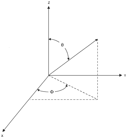
FIGURE 25.1 x,y,z coordinate system for NecWin modeling software.
Figure 25.2 depicts a single-wire antenna in free space. It has been laid out in model space centered on the origin (0,0,0) and extending from x = x1 (expressed as a positive number) to x = x2 (expressed as a negative number). In the more common case of an antenna close (in wavelengths) to an underlying ground such as earth, z at all points along the wire would be a positive, nonzero number if the wire represented a horizontal antenna. The wire in Fig. 25.2 has been placed where it is, relative to the three axes, for user convenience. There is no computational reason it couldn’t have also been placed along the y axis or at any angle in between the x and y axes. In fact, in free space, it could be at any angle and offset with respect to all three axes!
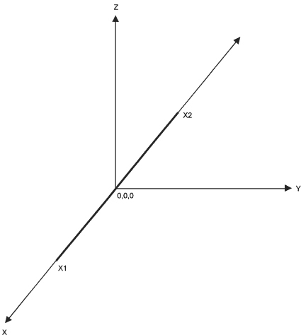
FIGURE 25.2 Example of a single wire laid out on x,y,z coordinate system.
In addition to its dimensions and location in model space, the antenna designer must specify how many segments each wire element is to be divided into and where any sources of RF current or voltage are to be located. Thus, the wire in Fig. 25.2 can serve as a center-fed dipole or an end-fed dipole or long wire, depending on where the feedpoint, or source, is located and the choice of measurement frequency. With practice, the user will learn how to quickly specify wires and their positions in model space, select an appropriate number of segments for each wire, and position sources within segments.
TIP When modeling antenna elements, such as dipoles, that are fed in the center, use an odd number of segments for the wire. This allows placement of the source or feedpoint in the exact center of the middle segment, thus duplicating the actual antenna very closely.
A Typical NEC-2 GUI
Roy Lewallen, W7EL, produces the EZNEC family of software for Windows PCs. The software extends Roy’s earlier work on DOS versions of EZNEC but is still based on the NEC-2 engine. (A professional version based on the NEC-4 engine is available for those who obtain the required government license.)
Figure 25.3A shows the opening screen in EZNEC+ ver 5.0 for a typical antenna project (in this case, an 80-m bent dipole). Visible in this window are file name, frequency, free-space wavelength (in meters), number of wires and segments, number of sources, number of loads, transmission lines, ground type, wire loss, the units employed (meters, feet, etc.), plot type (azimuth, elevation), elevation angle, step size, a reference level, and an alternate Z0 for the SWR plot (to conveniently handle both 50-and 75-Ω system impedances).

FIGURE 25.3A EZNEC+ ver. 5 opening screen.
Command buttons to the left of the main window include Open, Save As, Ant[enna] Notes, Currents, Src [Source] Dat[a], Load Dat[a], F[ar]Field] Tab[le], N[ear]F[ield] Tab[le], SWR, View Ant[enna], and F[ar]F[ield] Plot. The “FF Plot” button graphs the far field of the antenna as a function of azimuth (compass heading) for a given radiation (elevation) angle, or as a function of radiation angle for a user-selected azimuth (heading). Alternatively, the user can select a 3D presentation covering all elevations and azimuths in a single plot. Clicking on the “SWR” button brings up a new window for the user to define a frequency range and sample frequency intervals prior to running an SWR plot.
The wire and source tables used to create this antenna are shown in Fig. 25.3B. Note that the number of segments chosen for each of the three wires that make up the antenna keep the segment lengths as similar as possible. The horizontal wire in this example is divided into an odd number of segments to allow placement of a source at the exact midpoint of the center segment and, hence, at the midpoint of the antenna, in case it is to be a center-fed dipole. As can be seen from the rightmost two columns of the wire table, this antenna is being modeled with insulated wire.

FIGURE 25.3B Bent dipole wire and source tables.
The “View Antenna” window (Fig. 25.4) displays the x,y,z coordinate system and places all the wires specified in the Wires table according to coordinates entered there for each wire end. This window includes its own set of tools, including scroll bars to the left of the main window for zooming and repositioning the image within the window. Other options available from the drop-down menus include printer selection and setup, and a list of useful related objects (legends, currents, etc.) that can be displayed or not, as the user chooses. Once a set of calculations has been run, this window graphically shows (in a separate color) the magnitude of the current at all points on the antenna. A separate tabular listing of the current and its phase in each segment is also available for viewing, printing, or saving to a stand-alone file.

FIGURE 25.4 Bent dipole antenna view.
Once the user is satisfied by examination of the View Antenna display that all antenna data have been entered properly, pressing the “FF Plot” button in the main window opens a new window (Fig. 25.5) displaying the antenna’s far-field radiation pattern in the format previously determined by the choice of options in the main window. The plot shown here happens to be the radiated field versus azimuth (compass heading) for a bent dipole in free space (so the elevation angle is immaterial). Data entries beneath the plot display supporting information such as the elevation angle used for the calculation, the gain of the strongest lobe (wherever the pattern touches the 0-dB outer circle) over that of an isotropic radiator, front-to-back (F/B) ratio, beamwidth, and the azimuthal angle (listed as “Cursor Az”) for the strongest lobe. Alternatively, the user can opt to run an Elevation plot for a specific heading by making those selections and clicking on the “FF Plot” button again. The pattern will look different, of course, but the supporting data beneath it will be consistent with the first run.
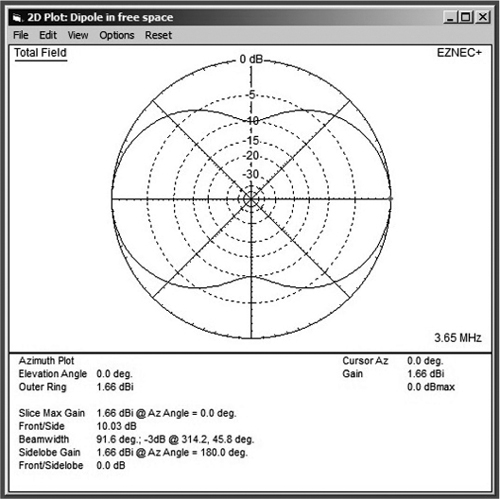
FIGURE 25.5 Bent dipole far field pattern.
NOTE Unless the antenna model is specified as being in free space, azimuth plots for a 0-degree elevation angle will return an error message for either of two reasons:
1. As discussed in Chap. 3, the presence of a perfectly conducting ground beneath a horizontally polarized antenna will result in zero radiated field at zero elevation angle because a voltage difference (an E-field, in other words) cannot exist between any two points on a lossless ground plane. When running azimuthal patterns for a horizontal dipole or Yagi over any kind of ground other than “free space”, choose a nonzero elevation angle (somewhere between 10 and 20 degrees, say) to see the low-angle azimuthal radiation pattern of the antenna. Cubical quads and loops fed in the center of their top or bottom sides should be handled the same way.
2. The resistive component of a “real” ground having finite conductivity will sap power from an advancing wavefront in contact with it, causing the zero elevation angle component of the wave to become nonexistent long before reaching a distant receiver. Again, when modeling any antenna type over one of NEC’s “real” ground options, choose a nonzero elevation angle to view the low-angle azimuthal radiation pattern of the antenna.
Recent versions of EZNEC include SWR plotting capability previously available only in the professional edition. Figure 25.6 shows the 50-Ω plot for the dipole under consideration. The displayed data include SWR, complex feedpoint impedance (Z), reflection coefficient, and return loss—all specified at the starting frequency or at any other stepped frequency within the plot range. Simply place your mouse pointer on the new frequency of interest and read off the (new) data below the graph.
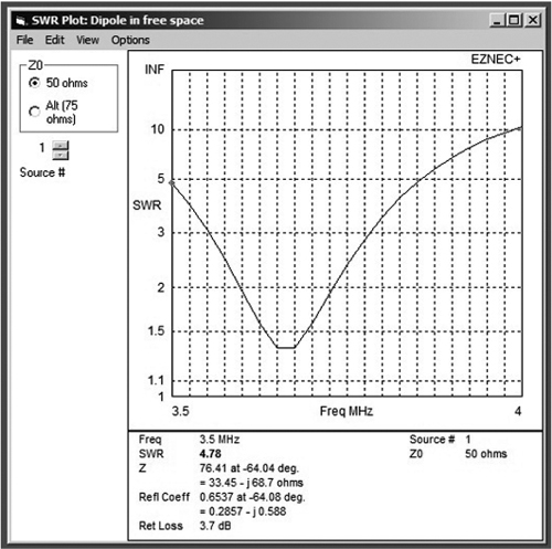
FIGURE 25.6 Bent dipole SWR plot.
Recently Added Features
Historically, the standard method of moments algorithms in NEC-based software for personal computers have not done a particularly good job with elements whose diameter changed at specified distances along the element, such as is almost always the case with HF beams. In recent years, however, special taper algorithms have been incorporated to correct that shortcoming. One example is an algorithm originally developed by David B. Leeson, W6ML (ex-W6QHS), in the process of mechanically strengthening a popular commercial HF Yagi. Recent versions of some user shells incorporate the Leeson taper algorithm, accessible as a menu option. To avoid confusion with a modeling technique called tapered segment lengths, the EZNEC menus, tables, and help files refer to the Leeson algorithm as stepped-diameter correction even though it has been a long-standing practice to call these tapered elements.
Another recent addition to many of the available programs is the ability to model a transmission line attached to the antenna. In some packages, commonly used “standard” transmission line models are already included and can be incorporated quickly into an otherwise custom antenna model. In general, the user must specify where on the modeled antenna each conductor at the antenna end of the transmission line connects, the line length and characteristic impedance (Z0), its velocity factor, and the loss per 100 ft at a user- or catalog-specified frequency. One benefit of this recent capability is that comparisons of parameters such as feedpoint impedance and SWR versus frequency between a model and its corresponding real antenna system can be performed from the comfort of the radio room.
An interesting feature of EZNEC 5 is the ability to optionally model two adjacent grounds of differing characteristics; the two grounds can even be at different heights! To access this capability, either of the “Real” types of ground (“High Accuracy” or “MiniNEC”) must first be selected. The user can then choose to have a single ground extending infinitely far in all directions or split the surface between two grounds in either of two ways: by a straight line dividing the grounds at a user-specified x coordinate or by a circle having a user-specified radius “R” where the ground characteristics change. The first option requires the user to rotate model space around the x and y axes until the model’s wires are oriented correctly with respect to the boundary between the two grounds, since this boundary is always parallel to the y axis. Both options provide an extremely useful feature for certain users . . . especially those who live near a body of water! The author’s antennas, for instance, are on a point of land approximately 10 ft higher than the freshwater lake that surrounds his property on three sides, so the circular boundary allows much better approximation of ground effects on his own antennas than a single ground does.
Other Considerations
One of the factors that serve to form practical limits on the capabilities of a given antenna modeling package is the number of wire segments needed to represent the antenna and neighboring conductors. For complex models (a Yagi beam in close proximity to other beams and wire antennas, for instance), the user may require an upgraded version of the software. Alternatively, judicious reduction in the number of segments used to model each wire may allow the model to run. As a general rule, however, it is good practice to think in terms of using 10 or more segments for each half-wavelength of wire length plus a few added segments wherever two wires meet at an angle or where two wires of different diameter are joined. The user can then fairly quickly add up the number of segments likely to be required for a multielement Yagi or quad.
Of course, the more segments in the model, the greater the number of computations that must be performed by the computer, although virtually any PC or Mac purchased within the past few years has more than enough “horsepower” for the inexpensive, segment-limited software packages that most of us are apt to purchase.
Although an “ideal” model of an antenna and the conductors around it would take into account all conducting structures in the vicinity of the target antenna, some common sense is required. For horizontal HF antennas there is likely to be little effect if vertical masts and lattice towers having horizontal dimensions less than λ/20 at the modeling frequencies of interest are not included. On the other hand, modeling an 80-m grounded vertical or a 40-m elevated ground-plane antenna within a wavelength of a 15-m or taller guyed tower supporting a triband Yagi might not yield accurate predictions unless the tower, Yagi, and metallic guy wires are added to the model.
Many “gotchas” are hidden in the inner workings of the NEC engine. So many, in fact, that antenna modeling should not be attempted without a thorough reading of the user manual that comes with each program. Even better is to take a course in the subject. ARRL, for instance, offers for a small fee a multisession online course that comes with an online tutor for the duration of the course and a substantial textbook for reference long after the course is completed. Examples and exercises in the ARRL book are split between EZ-NEC and NEC-Win Plus. The user is responsible for procuring his or her own copy of an appropriate modeling program prior to starting the course.
Perhaps the biggest “gotcha” for most users of these programs is the likelihood of serious inaccuracies in modeled performance of antennas that rely for their performance on one or more wires in contact with, or very close to, the ground. Over the years, each new version of the NEC core has improved in its ability to accurately describe the effects of nearby grounds and dielectrics on antenna performance. Current offerings based on the NEC-2 engine allow the user to select from as many as three different approaches to modeling the ground, and they contain an assortment of representative ground parameters for multiple soil types, freshwater lakes and ponds, seawater, and even custom permeability and dielectric constants defined by the user. Nonetheless, except for the more expensive packages built around the NEC-4 computing engine, all have a prohibition against modeling any wires in direct contact with the ground. As a result, grounded MF and HF verticals with extensive radial systems must be approximated by modeling the radials at a height of at least a few inches above ground. Model results for antennas based on the use of counterpoises (low wires running in close proximity to ground directly underneath the antenna wire) are similarly suspect, and the user should proceed with caution, reinforced with copious reading.
Once you have put together a model for your particular antenna, you should test the model for convergence—usually by making small changes to such things as the number of segments in each wire. A good model will yield results (maximum forward gain or feedpoint impedance, to name two examples) that vary by 1 percent or less with small changes in segment counts, wire diameters, etc. Discussion of all the techniques for confirming the quality of your model would be far more extensive than our limited treatment of antenna modeling has space for.
Terrain and Propagation Modeling Software
When modeling antennas, never lose sight of the fundamental objective: to maximize the ability to communicate via radio waves. Thus, while development of an optimized antenna is an important step, putting that antenna in the right location and/or at the right height can be just as important in sending those radio waves on their way.
While not strictly antenna modeling tools, two other categories of modeling software are especially germane to the process of optimizing signal paths between two stations for maximum received signal strength:
• Terrain analysis examines the effect of nearby (i.e., within a few miles) topographic features using principles of optical reflection and diffraction. In some countries, government or private topographical databases can be downloaded for automatic use by the software. If this is not the case in your country, manual entry is always possible. Terrain analysis is of great benefit when utilized prior to determining the height or location of antennas and their supports on a specific parcel of land, but it is probably of most benefit when used even earlier to compare the relative merit of multiple candidate sites for an antenna facility.
• Ionospheric propagation programs carry the ball the rest of the way, providing statistical predictions of optimum working frequencies, the probabilities and times for communicating between two points at any given time of the day, and the propagation modes providing the most efficient path between those points. In addition, some will predict received signal levels at distant receiving locations anywhere on the globe for a given transmitter power level.
See Chap. 2 (“Radio-Wave Propagation”) for additional information regarding these software tools.
Summary
Despite a plethora of caveats, “gotchas”, rules, and guidelines for users, today’s accurate yet inexpensive modeling tools are a boon to antenna experimenters everywhere. Hours or even days that might previously have been spent trudging through swamps, prickly brush, or deep snowdrifts to erect yet another configuration of wires atop the trees can now be put to better use, thanks to the power of the modern personal computer and the considerable efforts and accomplishments of a dedicated group of scientists, engineers, hobbyists, and entrepreneurs.
Many examples of antenna modeling results from both EZNEC (for the PC) and cocoaNEC (created by Kok Chen, W7AY, for the Mac) can be found in the chapters of this book dedicated to specific families of antennas. Any errors in the results presented are the fault of this author, not the software packages or their authors.
See App. B for a list of antenna modeling software vendors and the link for obtaining an NEC-4 license (U.S. users only).