CHAPTER 10
Wire Arrays
When a single wire gets substantially longer than a half-wavelength, or when multiple wires are employed, we enter the realm of wire arrays. In general, the purpose of using an array instead of a simpler antenna is to get higher forward gain, better rejection off the back and/or sides, or a combination of both. Few antenna projects bring as much reward at so low a cost as wires, and that’s especially true of wire arrays.
Longwire Antennas
The end-fed longwire (or, more simply, longwire) is a name given to any of several types of resonant and nonresonant antennas. The longwire antenna is capable of providing gain over a dipole and (if it is long enough) a low angle of radiation (which is great for DX operators!). But these advantages become substantial only when the antenna is several wavelengths long. Nonetheless, longwire antennas have been popular for decades—often because the layout of a particular property lends itself far more readily to locating one end of an HF wire close to the radio room, if not actually in it!
Any given longwire antenna may be either resonant or nonresonant, depending upon the operating frequencies used. In the old days, most longwires for use on the amateur MF and HF bands could be cut to be reasonably close to resonant on all the HF bands because those bands were harmonically related to each other. But with the addition of the 5-, 10-, 18-, and 24-MHz band segments, that’s not possible anymore.
Figure 10.1 shows the classic random length, nonresonant longwire antenna. It consists of a wire radiator that is at least a quarter-wavelength long but is most often much longer. The specific length is not critical, but by convention it is usually assumed to be a wavelength or more at the lowest frequency of operation anticipated. Nonetheless, a 70-ft wire fed at one end against a good RF ground will acquit itself well on all HF bands above 3.5 MHz.
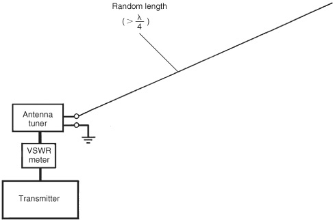
FIGURE 10.1 Random-length antenna.
The longwire is end-fed. Therefore, when it is an even number of quarter-wavelengths it will exhibit a very high feedpoint impedance (a few thousand ohms), while for lengths that are odd multiples of λ/4 it will present a much lower impedance (perhaps 25 to 100 Ω). Thus, it is imperative that an antenna tuner (ATU) be used, since even those transceivers with built-in antenna tuners typically cannot match the very high feedpoint impedances of end-fed wires that are approximately a multiple of λ/2 in length.
Often, the most important factor affecting the performance of an end-fed longwire is not the antenna—it’s the ground system it’s fed against! Although we may be aware that a λ/4 monopole radiates well only with the help of the ground system beneath it, any antenna with a single-wire feedline depends on the nearby ground to pass the return currents back to the transmitter circuits. If the transmitter is trying to push electrons into a longwire on each half-cycle of RF, it must necessarily be receiving or pulling an equal number of electrons from a return circuit of some kind. In the worst case, where no attention at all is paid to the ground return paths, the transmitter typically gets its return path from a mix of anything and everything that’s connected to the chassis and the ground of the power amplifier: ac power line, mic cable shield, audio cable shields, etc. Lack of attention to an appropriate ground return path is a major reason why equipment in a radio transmitting environment becomes “hot” whenever the transmitter is operated. The issue is especially relevant to the installation of a longwire antenna, since, in many cases, the fed end of the antenna actually comes right into the radio room.
Failure to include an adequate ground return for a longwire raises the apparent feedpoint impedance and causes a large portion of the transmitter output power to be dissipated in the resistive losses of other ground return paths rather than in the radiation resistance of the antenna. Ideally, many radials of lengths greater than or equal to λ/4 at the lowest frequency of operation, as shown in Fig. 10.2, should be included as part of any longwire antenna project.

FIGURE 10.2 Radials improve the “ground” of random-length antenna.
The kind of ground we’re talking about is not at all like the power company’s ground, which is a safety ground. The longwire requires an RF ground, which is discussed in detail in Chap. 30. At the very least, a λ/4 radial can be connected to the chassis of the ATU (or the transmitter if no ATU is used) and run outside. Of course, this effectively converts your longwire into an off-center-fed wire of unpredictable performance, but it’s far better than having no defined ground at all.
If you intend to use your longwire on more than one band, a single radial is of limited help. However, at least one company (MFJ) sells a tuner for the artificial ground. The MFJ model MFJ-931 artificial RF ground is installed between the radial wire and the ATU or transmitter chassis ground connection, as shown in Fig. 10.3. With every band change, the tuning controls will need to be adjusted for maximum ground current as indicated by the built-in meter. Keep in mind, however, that use of an artificial ground—with or without a tuner—falls in the category of trying to make the best of a bad situation.

FIGURE 10.3 MFJ ground line tuner installation.
Longwire Pattern and Gain
As the number of wavelengths in an end-fed wire increases—either by using a fixed-length wire on a higher frequency or by lengthening the wire while keeping the operating frequency fixed—both the pattern and the direction of maximum gain change, as well. At λ/2 the pattern of an end-fed wire is the broadside “doughnut” of a λ/2 dipole, perhaps very slightly skewed as a result of being fed at one end instead of in the center. At a length of λ, the doughnut-shaped figure eight pattern has broken into a four-lobed cloverleaf with peaks at 45 degrees from the antenna’s axis, and the maximum gain of the antenna (in the center of each lobe) has increased by almost 1 dB. As the frequency is further increased, the pattern breaks into more and more lobes, such as that depicted in Fig. 10.4 for a 2λ longwire, but the broadest of these maintain a gradual “march” toward the axis. At the same time, the peak amplitude of these main lobes gradually increases, reaching an additional 5 dB compared to the λ/2 wire at a length of 4λ, which corresponds to using an 80-m 135-ft λ/2 dipole on 10 m. Figure 10.5 plots the increase in gain of the main lobe relative to a λ/2 dipole as a function of longwire length.

FIGURE 10.4 Radiation pattern of longwire antenna.

FIGURE 10.5 Antenna length versus gain over dipole.
Regrettably, most longwires are fixed in one location; if the longwire is your only HF antenna, having the direction of peak signal gradually precess from broadside to nearly 90 compass degrees away while changing frequency may not suit your operating needs. More typically, however, an amateur or SWL with acreage available installs multiple longwires for a preferred band. An ideal configuration might have the fed end of all the wires located at a common point where an ATU is located and can be switched easily from one wire to another.
A rarely mentioned problem with very long wires: Electrostatic fields build up a high-voltage dc charge on longwire antennas! Thunderstorms as far as 20 mi away are known to produce substantial charge build-up on long antennas, capable of causing serious damage to a receiver or its operator! A simple solution is to connect a transmitter-rated RF choke (RFC) between the antenna terminal and the ground connection of the ATU. In a pinch, a dozen 10-MΩ, 2W resistors in parallel can be substituted.
Nonresonant Longwire Antennas
The resonant longwire antenna is a standing wave antenna because it is unterminated at the far end. A signal propagating from the feedpoint toward the open end will be reflected back toward the transmitter from the open end; the resulting superposition of the forward and reflected waves sets up stationary (i.e., “standing”) currents and voltages along the wire, similar to the process described in Chap. 3.
In contrast, a nonresonant longwire is terminated at the far end in a resistance equal to its characteristic impedance. (See Fig. 10.6.) Thus, the outward-bound wave is absorbed by the resistor, rather than being reflected. Such an antenna is called a traveling wave antenna. Terminating resistor R1 is selected to be equal to the characteristic impedance Z0 of the antenna (i.e., R = Z0). When the wire is 20 to 30 ft above average ground, Z0 is about 500 to 600 Ω.

FIGURE 10.6 Longwire (greater than 2λ) antenna is terminated in a resistance (typically 400 to 800 Ω). Radials under the resistor improve the grounding of the antenna.
The radiation pattern for the terminated longwire is a unidirectional version of the multilobed pattern found on the unterminated longwires. The orientation of the lobes varies with frequency, even though the pattern remains unidirectional. The directivity of the antenna is partially specified by the angles of the main lobes. It is interesting to note that gain rises almost linearly with nλ, while the directivity function changes rapidly at shorter lengths (above three or four wavelengths the rate of change diminishes considerably). Thus, when an antenna is cut for a certain low frequency, it will work at higher frequencies, but the directivity characteristic will be different at each end of the spectrum of interest.
Of course, if a terminated longwire is used for transmitting, approximately half the transmitter power will be dissipated in the termination resistor, so one should subtract 3 dB from the overall gain relative to unterminated antennas.
Arrays of Longwires
Longwire antennas can be combined in several ways to increase gain and sharpen directivity. Two of the most popular of these are the vee beam and the rhombic. Both forms can be made in either resonant (unterminated) or nonresonant (terminated) versions. Since a 1λ or longer longwire is itself an array, these antennas can be considered to be arrays of arrays.
Vee Beams
The vee beam (Fig. 10.7) consists of two equal-length longwire elements (Wire 1 and Wire 2), fed 180 degrees out of phase and oriented to produce an acute angle between them. The 180-degree phase difference is provided automatically by connecting the two wires of the vee to opposing sides of a single parallel conductor feedline.

FIGURE 10.7 Radiation pattern of vee beam antenna consists of the algebraic sum of the two longwire patterns that make up the antenna.
The unterminated vee beam of Fig. 10.7 has a bidirectional pattern that is created by summing together the patterns of the two individual wires. Proper alignment of the main lobes of the two wires requires an included angle, between the wires, of twice the radiation angle of each wire. If the radiation angle of the wire is β, then the appropriate included angle is 2β. To raise the pattern a few degrees, the 2β angle should be slightly less than these values. It is common practice to design a vee beam for a low frequency (e.g., 75-/80- or 40-m bands), and then to also use it on higher frequencies that are harmonics of the minimum design frequency. A typical vee beam works well over a very wide frequency range only if the included angle is adjusted to a reasonable compromise. It is common practice to use an included angle that is between 35 and 90 degrees, depending on how many harmonic bands are required.
Vee beam patterns are usually based on an antenna height that is greater than a half-wavelength from the ground. At low frequencies, such heights may not be possible, and you must expect a certain distortion of the pattern because of ground reflection effects.
The gain of a vee beam is about 3 dB higher than the gain of the single-wire longwire antenna of the same wire length, and it is considerably higher than the gain of a dipole (see Fig. 10.8). At three wavelengths, for example, the gain is 7 dB over a dipole. In addition, there may be some extra gain because of mutual impedance effects—which can be about 1 dB at 5λ and 2 dB at 8λ.
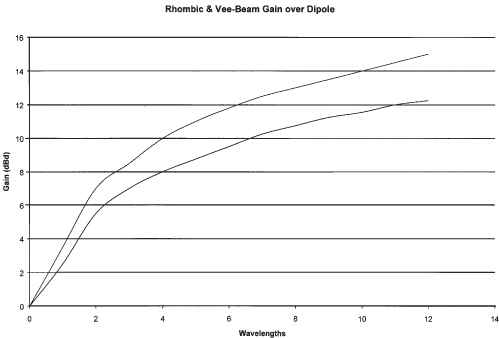
FIGURE 10.8 Gain versus length of vee beam and rhombic beam antennas.
Nonresonant Vee Beams
Like single-wire longwire antennas, the vee beam can be made nonresonant by terminating each wire in a resistance that is equal to the antenna’s characteristic impedance (Fig. 10.9). Although the regular vee is a standing wave antenna, the terminated version is a traveling wave antenna and is thus unidirectional. Traveling wave antennas achieve unidirectionality because the terminating resistor absorbs the incident wave after it has propagated to the end of the wire. In a standing wave antenna, any energy reaching the far end is reflected back toward the source, so it can radiate oppositely from the incident wave.

FIGURE 10.9 Nonresonant vee beam antenna.
Rhombics
The rhombic antenna, also called the double vee, consists of two vee beams positioned to face each other with their corresponding tips connected. The unidirectional, nonresonant (terminated) rhombic shown in Fig. 10.10 develops approximately the same gain and directivity as a vee beam of the same size. The nonresonant rhombic has a gain of about 3 dB over a vee beam of the same size (see Fig. 10.8 again).

FIGURE 10.10 Terminated rhombic antenna.
The layout of the rhombic antenna is characterized by two angles. One-half of the included angle of the two legs of one wire is the tilt angle (ϕ), while the angle between the two wires is the apex angle (θ). But the two are not independent; from Fig. 10.10 it should be obvious that θ/2 = 90 – ϕ. A common rhombic design uses a tilt angle of 70 degrees, a length of 6λ for each leg (two legs per side), and a height above the ground of 1.1λ. θ for this antenna must necessarily be 40 degrees.
The termination resistance for the nonresonant rhombic is 600 to 800 Ω, and it must be noninductive across the entire range of operating frequencies. For transmitting rhombics, the resistor should be capable of dissipating at least one-third of the average power of the transmitter. For receive-only rhombics, the termination resistor can be a 2W carbon composition or metal-film type. Such an antenna works nicely over an octave (2:1) frequency range.
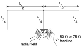
Bobtail Curtain
The bobtail curtain of Fig. 10.11 is a fixed array consisting of three individual quarter-wavelength vertical elements in a line; adjacent elements are spaced a half-wavelength apart and attached electrically to a horizontal wire across their tops that serves both as a phasing wire and as the other half of an L-shaped dipole. The array is fed at the bottom end of the center element. This is a high impedance point, so a parallel-tuned tank circuit or an ATU capable of matching very high impedances is required.
The array must be kept high enough in the air that the bottoms of the λ/4 vertical elements are some distance above ground—ideally high enough in the air that humans and animals cannot touch their high-voltage tips, although, clearly, the feed wire to the center element may require special protection. A bobtail curtain for 80 m should thus be suspended about 75 or 80 ft up; with catenary effects causing the phasing line to sag, end supports of at least 100 ft are appropriate.
RF energy introduced at the bottom of the center element splits and goes equally to the two end elements when it reaches the phasing line at the top. Since each end element is λ/2 from the center element, the currents of all three elements are in phase, although the current in the center element is twice that of either of the others. (This is an example of a 1:2:1 binomial array, as discussed in Chap. 5.) Since the currents feeding the two end elements are traveling in opposite directions along the top, and since the current to either end element goes through a reversal at the middle of the horizontal half-section, the horizontal radiation is partially canceled out.
Because all three elements are in phase, the principal lobe is broadside to the plane of the three radiating elements. For maximum signal north and south, for instance, the array should be suspended between supports on an east-west line.
The radiating elements are λ/4 monopoles and normally would require a low-resistance ground path for their return currents. However, if each vertical element is visualized as one side of a λ/2 dipole and half the horizontal distance along the phasing line to the adjacent element is seen as the other side of the dipole (or as an elevated groundplane), the vertical elements themselves have no particular need for a good ground system. However, unless there is an excellent RF ground at the base of the middle element for the matching network to connect to, there is no low-loss return path for RF currents flowing to/from the ground end of the matching network, and excessive transmitter power will be wasted in some vague but very lossy return path. Thus, the matching network at the base of the middle element may require a good system of radials. Since radials lying on the surface of the earth are not resonant, their exact length is not particularly critical. It might be helpful, depending on the quality of your ground, to put radial fields under the end elements, as well.
The bobtail curtain has an extremely low angle of radiation. At one time the author had an 80-m bobtail curtain aimed north and south at his home in the northeastern United States; it was a “killer” antenna for very long haul contacts over the north pole into the far reaches of Asiatic Russia and the western Pacific region—especially Indonesia—but it was totally useless for anything much closer.
Half-Square
If one end element of the bobtail curtain of Fig. 10.11 and its associated phasing line are removed, the resulting antenna is known as a half-square. Now we have two vertical radiators joined by a λ/2 horizontal phasing line. As with the original bobtail curtain, the antenna is fed at the bottom of one element—a high impedance point. (Keep in mind that both the fed end and the far end are high-voltage points.) We can consider that element and half the horizontal wire as constituting an L-shaped λ/2 dipole feeding a second λ/2 dipole. But since the current in consecutive λ/2 sections reverses, the instantaneous current in the second vertical element is always pointed in the same direction—up or down—as that of the first.
Thus the half-square is a two-element broadside array. If it is hung from east and west supports, maximum radiation is north and south. Off either end, contributions by the two vertical radiators are 180 degrees out of phase, thanks to the λ/2 spacing between them, so the array has a null to the east and west. Because the currents in the two halves of the horizontal wire are also out of phase, they mostly cancel and the array exhibits relatively little high-angle radiation.
Over average ground, the half-square has about 4 dB additional gain broadside to the axis of the antenna compared to a single λ/4 vertical, and the peak of the main lobe occurs at a lower elevation angle (20 degrees versus 23 degrees). As before, each λ/4 vertical monopole can utilize half the horizontal wire as a radial, but overall system efficiency and the specifics of the matching network may dictate the use of radials directly connected to the ground and chassis of the ATU that feeds the vertical wire. Adding radials under both vertical elements adds about 0.4 dB to the low-angle broadside gain over average earth.
20-m ZL-Special Beam
The antenna shown in Fig. 10.12 is a close relative of the Yagi beam. It consists of a pair of folded dipoles mounted approximately 0.12 wavelengths apart. Each element is 30.5 ft in length, and the spacing between the two is 7.1 ft. Each element can be made of two parallel wires separated with spacers or from 300-Ω television-type twin lead. Alternatively, if the antenna is to be rotatable, wires inside small PVC tubes supported at their ends by a truss assembly can be used, as can spaced aluminum tubing.

FIGURE 10.12 ZL-special beam antenna.
The two λ/2 folded dipole elements of the ZL-special are fed 135 degrees out of phase with respect to each other. The feedline is connected to one of the dipoles directly; the other is fed through a length of 300-Ω twin lead that has an electrical length of about 45 degrees (λ/8) and has been given a half-twist to add another 180 degrees of phase shift. Its physical length will depend on the velocity factor vF of the particular line used.
The feedpoint impedance is on the order of 100 to 150 Ω, so the antenna is a good match for either 52-Ω or 75-Ω coaxial cable if a 2:1 impedance matching transformer is used.