Where to Go from Here Solutions
Solutions for the exercises in Try Your Hand.
-
The truth table for the constant function
 is:
is:


-
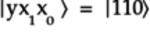
From the truth table in the previous part, when the bottom qubit
is , the state
 is , and vice versa.
In other words, the
is , and vice versa.
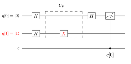
In other words, the  block is a pass-through
for the top qubit and acts like a NOT (X) gate
for the bottom qubit. The resulting Deutsch circuit is
shown in the following figure:
block is a pass-through
for the top qubit and acts like a NOT (X) gate
for the bottom qubit. The resulting Deutsch circuit is
shown in the following figure:
-
The Qiskit program for this circuit is listed below:
1: # import Qiskit and other libraries - import numpy as np - import math - from qiskit import( 5: QuantumCircuit, - QuantumRegister, - ClassicalRegister, - execute, - Aer) 10: from qiskit.visualization import plot_histogram - - # Set up circuit with 2 qubits and 1 classical register - circuit = QuantumCircuit(2,1) - circuit.x(1) 15: circuit.h(range(2)) - circuit.x(1) - circuit.h(0) - circuit.measure(0,0) # Measure gate on top qubit - circuit.draw(output='mpl') 20: - # Get Backend and run circuit - backend = Aer.get_backend('qasm_simulator') - job = execute( circuit, backend, shots=1 ) - 25: # plot results - hist = job.result().get_counts() - plot_histogram( hist ) Note the NOT (X) gate on line 14 to set the bottom qubit to
before splitting it by the H gate.
On line 23 the number of shots is set to 1.
After running this program, the Measure gate on the top qubit records a 0 in the classical register indicating that the function
 is constant.
-
The Cirq program for this circuit is listed here:
1: # Import Cirq libraries - import cirq - from cirq.ops import H, X - 5: # Declare the qubits - place diagonally: q[0] at (0,0), q[1] at (1,1) - q = [cirq.GridQubit(i, i) for i in range(2)] - - # Set up Circuit - circuit = cirq.Circuit() 10: circuit.append([X(q[1]),H(q[0]), H(q[1]), X(q[1]), H(q[0])]) - circuit.append(cirq.measure(q[0], key='m')) - - print(circuit) - 15: # Get a simulator to execute the circuit - simulator = cirq.Simulator() - # Simulate the circuit several times - result = simulator.run(circuit, repetitions=1) - # Print the results 20: print("Results:") - print(result) On line 6, declare the qubits and place them diagonally at (0,0) and (1,1) on the grid.
On line 18, the number of shots is set to 1.
After running this program, you’ll find that the Measure gate on the top qubit records a 0, indicating that the function is constant.
-
Both circuits return identical results when run on the IBM and Google Quantum Computers, respectively. In each case, just a single shot confirms that the function is constant.
-
-
The truth table for the balanced function
is:
-
To figure out the
block for this
balanced function, first work
out the matrix based on the truth table you
determined in the previous part.
The state of the qubits on the left of the
, and ,
map to those on the right, and
 ,
as follows:
,
as follows:
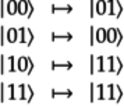
In other words, the matrix
 for is:

With a little bit of experimentation, you’ll come up with the arrangement of the CNOT and NOT (X) gates, as shown in the following figure:

-
The Qiskit program for this circuit is listed here.
1: # import Qiskit and other libraries - import numpy as np - import math - from qiskit import( 5: QuantumCircuit, - QuantumRegister, - ClassicalRegister, - execute, - Aer) 10: from qiskit.visualization import plot_histogram - - # Set up circuit with 2 qubits and 1 classical register - circuit = QuantumCircuit(2,1) - circuit.x(1) 15: circuit.h(range(2)) - circuit.cx(0,1) - circuit.x(1) - circuit.h(0) - circuit.measure(0,0) # Measure gate on top qubit 20: circuit.draw(output='mpl') - - # Get Backend and run circuit - backend = Aer.get_backend('qasm_simulator') - job = execute( circuit, backend, shots=1 ) 25: - # plot results - hist = job.result().get_counts() - plot_histogram( hist ) The bottom qubit is initialized to
by the X gate on line
14.
On line 24 the number of shots is set to 1.
After running this program, the Measure gate on the top qubit records a 1 in the classical register, indicating that the function
is balanced.
-
The Cirq program for this circuit is listed below:
1: # Import Cirq Libraries - import cirq - from cirq.ops import CNOT, H, X - 5: # Declare qubits-place one below the other: q[0] at (0,0) & q[1] at (1,0) - q = [cirq.GridQubit(i, 0) for i in range(2)] - - # Set up Circuit - circuit = cirq.Circuit() 10: circuit.append([X(q[1]),H(q[0]), H(q[1]), - CNOT(q[0],q[1]), X(q[1]), H(q[0])]) - circuit.append(cirq.measure(q[0], key='m')) - - print(circuit) 15: - # Get a simulator to execute the circuit - simulator = cirq.Simulator() - # Simulate the circuit several times - result = simulator.run(circuit, repetitions=1) 20: # Print the results - print("Results:") - print(result) On line 6, declare the qubits and place them one below the other at (0,0) and (1,0) on the grid.
On line 19 the number of shots is set to 1.
After running this program, you’ll find that the Measure gate on the top qubit records a 1, indicating that the function is balanced.
-
Both circuits return identical results when run on the IBM and Google Quantum Computers, respectively. In each case, just a single shot confirms that the function is balanced.
-
-
Since for half the input states, the function returns
and for the
other half returns ,
the function  is balanced.
You would need to sample three times
to establish its type.
is balanced.
You would need to sample three times
to establish its type.
-
The
block is shown in the following
figure:

-
The truth table for
is as follows:


-
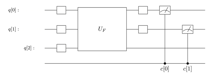
The quantum circuit for the Deutsch-Jozsa algorithm to test the type of a two-qubit function is shown in the following figure:
-
To figure out the matrix
 for
this truth table, work out the quantum state vector
for each of the idealized states, but label the states
in the IBM convention. That is, write the quantum
state as a concatenated string of the states in
the quantum registers
for
this truth table, work out the quantum state vector
for each of the idealized states, but label the states
in the IBM convention. That is, write the quantum
state as a concatenated string of the states in
the quantum registers  :
:
- Idealized state
 :
: -
The output quantum state is
 .
In vector form:
.
In vector form:

This vector is the first column of
.
- Idealized state
 :
: -
The output quantum state is
 .
In vector form:
.
In vector form:

This vector is the second column of
.
- Idealized state
 :
: -
The output quantum state is
 .
In vector form:
.
In vector form:

This vector is the third column of
.
- Idealized state
 :
: -
The output quantum state is
 .
In vector form:
.
In vector form:

This vector is the fourth column of
.
- Idealized state
 :
: -
The output quantum state is
 .
In vector form:
.
In vector form:

This vector is the fifth column of
.
- Idealized state
 :
: -
The output quantum state is
 .
In vector form:
.
In vector form:

This vector is the sixth column of
.
- Idealized state
 :
: -
The output quantum state is
 .
In vector form:
.
In vector form:

This vector is the seventh column of
.
- Idealized state
 :
: -
The output quantum state is
 .
In vector form:
.
In vector form:

This vector is the eighth column of
.
Thus, the matrix
is:

- Idealized state
-
The quantum program using Qiskit is listed here:
1: import numpy as np - import math - from qiskit import( - QuantumCircuit, 5: QuantumRegister, - ClassicalRegister, - execute, - Aer) - from qiskit.visualization import plot_histogram 10: from qiskit.quantum_info.operators import Operator - - - U_F = Operator([ - [1,0,0,0,0,0,0,0], 15: [0,0,0,0,0,1,0,0], - [0,0,1,0,0,0,0,0], - [0,0,0,0,0,0,0,1], - [0,0,0,0,1,0,0,0], - [0,1,0,0,0,0,0,0], 20: [0,0,0,0,0,0,1,0], - [0,0,0,1,0,0,0,0] - ]) - - 25: # Check unitary - print('Operatator is unitary:', U_F.is_unitary()) - - circuit = QuantumCircuit(3,2) - circuit.x(2) 30: circuit.h(range(3)) - circuit.append(U_F,[0,1,2]) - circuit.h(range(2)) - circuit.measure([0,1],[0,1]) - 35: circuit.draw(output='mpl') - - # Use simulator to run the circuit - backend = Aer.get_backend('qasm_simulator') - # Define the run parameters and execute 40: job = execute( circuit, backend, shots=1 ) - # Tally the results - collapsed_states_array = job.result().get_counts() - print(collapsed_states_array) The matrix
is defined on
lines 13--22
using Operator. (To use this method,
you have to first import it on
line 10.)
Set up the circuit on lines 28--33.
The “gate” corresponding to the matrix
is appended to the
circuit on line 31.
On line 38
select the simulator to run this program. And on line
40,
specify to run only once. Get the collapsed state on
line 42.
-
The output of this program is:
{'01': 1} Since the output state isn’t 00, indicating that the function is not constant, it, therefore, must be balanced.
-
-
The first choice correctly assigns H gates to all three qubits.
The second choice, circuit.h(3), throws an error as the system will try to assign an H on q[3], which is out of range. The circuit was initialized with three qubits: q[0], q[1], and q[2].
The third choice, circuit.h(0,1,2), has three arguments. The h method only allows a single argument: either the index of the qubit on which to place the H gate, or an array of qubits on which the H gates are placed.
The fourth choice, h.(range(2)), will assign H gates to only the first and second qubits, not all three.
-
The last choice correctly assigns H gates on both qubits and places the Measure gates on the qubits.
The first choice, circuit.measure(range(2),range(2)), works out to circuit.measure([0,1],[0,1]). That is, the Measure gate on the first qubit records the collapsed state in c[0], the first classical register, and the Measure on the second qubit records it in c[1]. The given circuit has it the other way around: the collapse of the first qubit is recorded in c[1], the second classical register, and the collapse of the second qubit is recorded in c[0], the first classical register.
The second choice throws an out-of-range error as the assignments of both the H gate and Measure gates use indices that are outside the range declared.
The third choice only assigns a single Measure gate that records the collapse of the second qubit in the first classical register. The circuit has two Measure gates.
-
-
This gate splits and rotates the triangle
qubelets. So the last description best describes the
gate.
-
Yes. The amplitude includes the complex number
 , which indicates that the triangle
qubelets are rotated
90° anticlockwise. (See
Rotating Qubelets Through Any Angle,
for the definition of the quantum state.)
, which indicates that the triangle
qubelets are rotated
90° anticlockwise. (See
Rotating Qubelets Through Any Angle,
for the definition of the quantum state.)
The probability that the
qubit collapses to is
calculated as shown below:

-
Yes. The amplitude includes the complex number
 , which indicates that the triangle
qubelets are rotated
90°clockwise. (See
Rotating Qubelets Through Any Angle,
for the definition of the quantum state.)
, which indicates that the triangle
qubelets are rotated
90°clockwise. (See
Rotating Qubelets Through Any Angle,
for the definition of the quantum state.)
The probability that the
qubit collapses to is
calculated as shown below:

Notice that when working with complex numbers, “squaring the amplitude” is replaced by multiplying it with its complex conjugate.
-
When this gate acts on the
qubit, the quantum state written as a vector is:
This vector becomes the first column of the gate’s matrix
 .
.
When this gate acts on the
qubit, the quantum state written as a vector is:

This vector becomes the second column of the gate’s matrix
.
Thus, the matrix
for this gate is:

-
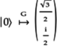
To check whether the
matrix is
unitary, write a program using Qiskit as follows:
1: import numpy as np - import math - from qiskit import( - QuantumCircuit, 5: QuantumRegister, - ClassicalRegister, - execute, - Aer) - from qiskit.visualization import plot_histogram 10: from qiskit.quantum_info.operators import Operator - - A_G = [ - [math.sqrt(3)/2, 1/2*complex(0,1)], - [1/2, -math.sqrt(3)/2*complex(0,1)] 15: ] - - gate_G = Operator(A_G) - - print('Operatator is unitary:', gate_G.is_unitary()) On line 10, import the Operator library. Define the
matrix on line 12.
To make this matrix a quantum gate, pass it in an
argument to the Operator object
on line 17.
And then, on line 19,
check whether the matrix is unitary.
Running this code will return True, indicating that the
matrix is
unitary and can be safely used as a gate in a quantum
circuit.
-
Add the following lines to the program in the previous part to set up the circuit and run it on the simulator:
1: # Set up circuit 2: circuit = QuantumCircuit(2, 2) 3: circuit.append(gate_G, [0],) 4: circuit.x(1) 5: circuit.cx(0,1) 6: circuit.measure([0,1], [0,1]) 7: 8: circuit.draw(output='mpl') On line 2, declare a circuit having two qubits and two classical registers. Then, on line 3 insert the G gate you just defined, followed by the rest of the gates that make up the circuit.
-
To run the circuit on the simulator, append the following lines to the Qiskit code in the previous part:
1: # Select Simulator 2: backend = Aer.get_backend('qasm_simulator') 3: 4: # Define the run parameters and execute 5: job = execute( circuit, backend, shots=1024 ) 6: 7: # Tally the results 8: collapsed_states_array = job.result().get_counts() 9: print(collapsed_states_array) On lines 2--9, set the program to run on a simulator and print the results as an array.
After you run this circuit on the simulator, the two qubits will collapse roughly into the following two states:
{'10': 763, '01': 261} In fact, these qubits are entangled. If you see 1 in c[0], you’re guaranteed to see 0 in the other classical register, and vice versa. As the counts over the 1024 repetitions show, you’ll see 0 in c[0] about three times as often you’ll see 1. (Remember that the order of the classical registers in IBM’s Quantum Computer is reversed from the way we’ve labeled them. That is, the right-most bit corresponds to c[0].)
-
Yes, you could have defined the matrix as a U3 Universal gate.
-
-
No. The sum of probabilities of collapsing to the four idealized states is:

Since this sum doesn’t add up to 1, the quantum state
 is not valid.
To make this quantum state valid, normalize it as follows:

-
The Qiskit program that initializes the circuit with
is listed
here:
1: import numpy as np - import math - from qiskit import( - QuantumCircuit, 5: QuantumRegister, - ClassicalRegister, - execute, - Aer) - from qiskit.visualization import plot_histogram 10: from qiskit.quantum_info.operators import Operator - - input_quantum_state = [ 1/math.sqrt(15), - -2/math.sqrt(15), - 3/math.sqrt(15), 15: -complex(0,1)/math.sqrt(15) - ] - - # Define circuit with 3 qubits and 3 classical registers - q = QuantumRegister(3) 20: c = ClassicalRegister(3) - circuit = QuantumCircuit(q,c) - circuit.initialize(input_quantum_state, [q[0],q[1]]) - - circuit.h([q[0],q[2]]) 25: circuit.cx(0,1) - circuit.h(0) - circuit.cx(2,1) - circuit.measure(q, c) - 30: circuit.draw(output='mpl') The quantum state
is defined on
line 12.
On line 22
the circuit is initialized with the quantum state
. The gates are declared on
lines 24--28.
-
To determine the number of independent states, use the num_unitary_factors of the circuit object:
circuit.num_unitary_factors() Since, the two CNOT gates entangle all three qubits, there’s only a single independent set of qubits.
-
To run the circuit on the simulator, append the following lines to the Qiskit code in the previous part:
backend = Aer.get_backend('qasm_simulator') # Define the run parameters and execute job = execute( circuit, backend, shots=1024 ) # Tally the results collapsed_states_array = job.result().get_counts() print(collapsed_states_array) The output of this circuit reported as an array will be similar to the following:
{'001': 158, '111': 147, '101': 5, '000': 28, '100': 308, '011': 7, '110': 36, '010': 335} You can also plot these states as a histogram with the following line:
plot_histogram( collapsed_states_array )
-
-
The list of quantum effects includes the following:
- Superposition.
-
Rotating pentagon and
triangle qubelets.
- Canceling qubelet combinations.
- Entangling qubelets.
- Back-to-back H gates for restoring states.