Multi-Qubit Superposition: The Mega-Qubit
Controlling randomness is, without doubt, an essential ingredient for quantum computing. But quantum computing offers an even more compelling case for reinventing computing. It gives us a way to deal with the entire solution space as a single unit. This may sound intimidating, but we’ll learn that to think about the entire solution space at once, we must focus on the characteristics a solution obeys rather than on the individual solutions themselves. So, before designing quantum algorithms that find a solution to a system of Boolean expressions, we need to first get comfortable with this shift in mindset.
Parallel H Gates
For our next exercise, we’ll deal with two qubits and learn how to grapple with all-solutions-at-once. We’ll start with the following circuit with two qubits:

Here’s the code, excluding the header, for this circuit:
| | qreg q[2]; |
| | creg c[2]; |
| | |
| | // Put qubits in superposition |
| | h q[0]; |
| | h q[1]; |
| | |
| | measure q[0] -> c[0]; |
| | measure q[1] -> c[1]; |
Each qubit is initialized to ![]() and
acted on by the H gate. This puts
each qubit in a superposition, as shown here:
and
acted on by the H gate. This puts
each qubit in a superposition, as shown here:
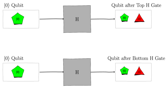
If we feed these qubits to other gates, then those other gates will operate on blended qubits. To put it another way, those gates will operate on the various combinations formed by the qubelets in the top and bottom qubits. We represent these combinations of qubelets as a mega-qubit, as shown in the following figure:
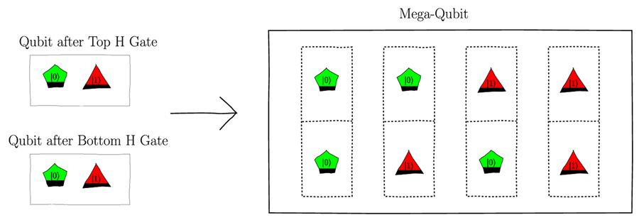
In each combination, or column, of qubelets in the mega-qubit on the right, the top qubelet is from the top qubit, and the bottom qubelet from the bottom qubit. The qubelets on the top represent the quantum state of the top qubit, and those on the bottom represent the bottom qubit. Thus, each column is a possible state of the qubits. In this case, the mega-qubit has four states: ⎹00⟩, ⎹01⟩, ⎹10⟩, and ⎹11⟩, where the first digit is the top qubit and the second one is the bottom qubit.
Mega-Qubit Is the Quantum State of System | |
|---|---|
|
|
The mega-qubit models the quantum state of the system. It’s an aggregate of the entire set of qubelet columns, each of which represents a possible value of the qubits in the circuit. The mega-qubits used to analyze the behavior of qubits, however, are a mental device to help us analyze quantum circuits and write programs that properly harness quantum behavior. They’re not real, at least not in the traditional sense. No one really knows what happens at the quantum level. So the mega-qubit serves as a stand-in for subatomic phenomena that helps us arrive at results that can be verified. |
Even though we’ve drawn the mega-qubit holding four distinct combinations or columns of qubelets, in reality they are all presented simultaneously to the subsequent gates as blended qubits. The mega-qubit, in fact, represents the state of the entire system and is the key to how quantum computers solve problems. Thus, you may think of a quantum computer as a massively parallel processor running on jet fuel.
When we run this circuit, after passing the top and bottom qubits to the H gate, we measure them, thereby collapsing them. Measuring the qubits is equivalent to first selecting a qubelet combination, or column, at random from the mega-qubit and then recording the corresponding binary bits. So we’ll see each of the four cases—00, 01, 10, and 11—roughly 25% of the time, as shown here:

Note that as per the quantum circuit, we’re recording the collapsed state of q[0] in c[0] of the classical register and that of q[1] in c[1]. Thus, in each string of qubits at the bottom of the bars in the output, the left character corresponds to the classical state that the qubit in q[1] collapses to, and the right character is the binary state of the collapsed qubit in q[0].
Operating on Mega-Qubits
To see how a quantum computer deals with a mega-qubit, consider the following quantum circuit:

The code for this circuit is the following:
| | qreg q[2]; |
| | creg c[2]; |
| | |
| | h q[0]; |
| | cx q[0],q[1]; |
| | measure q[0] -> c[0]; |
| | measure q[1] -> c[1]; |
After the top qubit is operated on by the H gate, the qubits will be in the quantum states shown here:

This blended qubit is put into a
superposition with the bottom ![]() qubit:
each qubelet in the top qubit pairs up with the
single pentagon
qubit:
each qubelet in the top qubit pairs up with the
single pentagon ![]() qubelet in the
bottom qubit to form the following mega-qubit:
qubelet in the
bottom qubit to form the following mega-qubit:

The top qubelets in each column are associated with the q[0] qubit, and the bottom qubelets are associated with the q[1] qubit.
When this mega-qubit is operated on by the CNOT gate, all the qubelet combinations are simultaneously operated on by the CNOT gate. Even though all the qubelet combinations are acted on all at once, to work out what the new mega-qubit would look like, we apply the CNOT gate individually on each qubelet combination. As we saw in Controlled NOT (CNOT) Gate, the CNOT gate leaves ⎹00⟩ as is but changes ⎹10⟩ to ⎹11⟩. Thus, the mega-qubit after applying the CNOT gate is shown here:
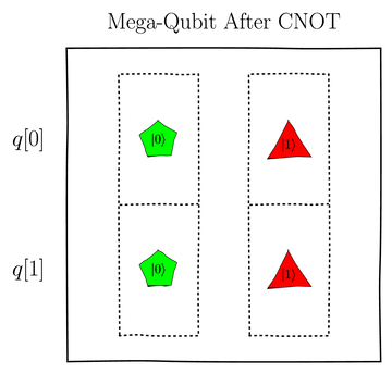
If we now measure the control and target qubits, one of the two qubelet combinations in the mega-qubit would be randomly selected with equal probability. Thus, we would see the states 00 or 11 roughly equally. Specifically, the output of the program is shown in the following figure:

Taming the Mega-Qubit Explosion: A Sneak Peek
While the mega-qubit model gives us a way to think about quantum superposition, it introduces a significant challenge: with two qubits, we get four pairs of qubelet combinations or columns; with three qubits, we get eight combinations; and with n qubits we get 2n combinations. For large problems, this situation rapidly becomes unmanageable when designing quantum programs. The hardware won’t break a sweat, but writing and thinking about code in the classical way becomes impractical.
Quantum programming takes a different approach. Instead of focusing on writing software that steers each combination through the program individually, in quantum programming our objective will be to identify the characteristics of a solution and then configure gates to cull the quantum states that don’t play a role in solving the computational task. We won’t know what the optimal solution is to a computational task when we write the code, we will know that the Boolean constraints have to be met. Specifically, we’ll see how the Z gate, which we study in Chapter 5, Beam Me Up, Scotty—Quantum Tagging and Entangling , inverts qubelets to cancel out the unwanted states. We’ll get into the details later, but I wanted to give you at least a glimpse of the path forward. Next we’ll review how to put the qubits in a quantum circuit into superposition.