Measuring Qubits
Having settled on an understanding of qubits and quantum states, we’re ready for the next step in our journey. To get anything useful out of qubits, we control them with quantum gates, the quantum equivalent of classical gates.
To get a feel for quantum programs steering quantum states to the correct solution, imagine a magic trick where your selected card appears at the top of the deck. It may look random, but the shuffling of the deck is actually a controlled reordering of the cards to force the selected card to the top of the deck. Likewise, even though the quantum bits collapse randomly to one of the two idealized states, the quantum program applies the quantum gates in a way that forces the qubits to collapse to the desired state.
Because quantum gates guide qubits to reliably transition from one quantum state to another, they work differently from the classical gates. You can’t simply take the code you wrote for a conventional computer and run it on a quantum computer. In fact, because of the unique way that quantum gates work, you’ll need to redesign your logic circuit, the interconnection of classical logic gates to perform a computational task, and, thus, your program, so that you get the qubits to simultaneously collapse to binary states that correspond to an optimal solution, as we saw in A Scheduling Problem. In quantum computing, the interconnection of quantum gates is called a quantum circuit.
Quantum Circuits Are Wireless | |
|---|---|
|
|
Even though we draw quantum logic circuits with wires connecting the quantum gates, you shouldn’t think that qubits flow through them as electrons would. The wires in a quantum circuit aren’t physical as they are in electronic circuits. Rather, you should think of the wires as a conveyor belt that brings the quantum gates in the order drawn in the circuit to act on the qubit. |
Before we string quantum gates together to build a complete program, you must first learn how quantum gates behave individually so that you understand how to rework your application’s logic circuit. We’ll start with the Measure gate. Every quantum program you write needs these.
Measure Gate
In the previous section we saw that since quantum states can’t be directly observed, the only thing that a quantum program can disclose is the collapsed states of qubits. So although we’ll write programs that intelligently vary the quantum states of qubits to arrive at states that correspond to an optimal solution, we have to eventually collapse the qubits to obtain the associated binary states. Hence, before studying other gates and quantum statements, we must first know how to read the result of a quantum computation that changes a qubit’s quantum state. That is, we need a way to collapse a qubit’s quantum state in code.
The Measure gate is a quantum instruction that collapses a qubit: it randomly selects a qubelet from the qubit and returns the state of the selected qubelet. The returned state is a classical binary state. Conceptually, the Measure gate is shown in the following circuit:

The left qubit has two pentagon ![]() qubelets and three triangle
qubelets and three triangle ![]() qubelets.
The Measure gate randomly selects a
qubelet, for example, a pentagon
qubelets.
The Measure gate randomly selects a
qubelet, for example, a pentagon ![]() qubelet, from the left qubit. The left qubit is collapsed
to
qubelet, from the left qubit. The left qubit is collapsed
to ![]() and the returned classical
state is 0.
This act of collapsing a qubit is called measuring
or examining the qubit.
and the returned classical
state is 0.
This act of collapsing a qubit is called measuring
or examining the qubit.
Under the hood, the process works a little differently. So let’s fix the figure above. After collapsing the qubit, the Measure—the binary value corresponding to the idealized quantum state—is recorded in a register. By convention, this recording action is depicted as shown in the circuit.
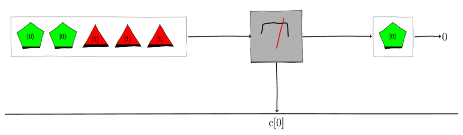
The down arrow is the Measure gate writing to a standard classical register on the bottom horizontal line.
A Measure gate records the binary state of the collapsed qubit, which forms the output of your quantum program. Thus, you can think of the Measure gate as your program’s return statement.
Selecting a Qubelet Is Measuring a Qubit | |
|---|---|
|
|
The process of randomly selecting a qubelet, collapsing the qubit by getting rid of the other qubelets in the quantum state, and recording the state of the selected qubelet as a binary bit is called measuring a qubit.
For example, when we say that the Measure
gate collapses the qubit to 0, it’s
shorthand for the Measure gate
selecting a pentagon |
It shouldn’t escape your attention, though, that unless
you’re writing a random number generator, collapsing
the qubit on the left with two pentagon ![]() qubelets and three triangle
qubelets and three triangle ![]() qubelets
is premature: sometimes you’ll end up with a 0
and at other times a 1 in the classical register.
The challenge in quantum
computing is to coax qubits to quantum states that
have an extremely high likelihood of collapsing
to the optimal binary states so that you don’t end up
logging random states when you measure the qubits.
Before seeing how to work with qubits in a program,
we’ll start by covering how to use a Measure
gate in code.
qubelets
is premature: sometimes you’ll end up with a 0
and at other times a 1 in the classical register.
The challenge in quantum
computing is to coax qubits to quantum states that
have an extremely high likelihood of collapsing
to the optimal binary states so that you don’t end up
logging random states when you measure the qubits.
Before seeing how to work with qubits in a program,
we’ll start by covering how to use a Measure
gate in code.
Writing the Quantum Program
To declare a Measure gate in a quantum program, we’ll build the following circuit:

This circuit has a single qubit held in the quantum register q[0], and a single classical register, c[0], where the Measure gate records the binary bit associated with the collapsed quantum state of the qubit.
To write a program for this circuit, go to the IBM Quantum Computer and click the Create a circuit button. This opens the Circuit Composer, where you can connect the gates for the circuit as shown in the following figure:

The Circuit Composer initializes five quantum registers and five classical registers. Our circuit, though, only has a single qubit and a single classical register. To remove the extra qubits and classical registers, go to the Composer Home panel on the left and click the Circuit editor tab. In the Circuit editor panel, you’ll see the following initial code:
| ① | OPENQASM 2.0; |
| ② | include "qelib1.inc"; |
| | |
| ③ | qreg q[5]; |
| ④ | creg c[5]; |
Every quantum program begins with the headers shown on the first two lines followed by the code that specifies the quantum circuit:
- ①
-
Specify the version of the Quantum Assembly Language used for the quantum program.
- ②
-
Reference the include file that contains pre-built functions for the quantum instructions.
- ③
-
The keyword qreg declares the 0-based quantum register array that holds the qubits. The default name for this array is q, but you can change it to another label if you’d like. The length of the array is the number of qubits you’ll use in your program. All qubits are initialized to
 .
Later, we’ll learn how to initialize it to
.
Later, we’ll learn how to initialize it to
 and other blended
states.
and other blended
states.
- ④
-
The keyword creg declares the 0-based classical register array that holds the binary values of the collapsed qubits. The default name for this array is c, but you can change it to another label if you’d like. The length of this array is the number of collapsed qubits you want your program to return.
To get rid of the extra qubits and classical registers, set their lengths to 1:
| | qreg q[1]; |
| | creg c[1]; |
To connect the Measure gate to the qubit in q[0], drag it from the palette to the top line, representing the qubit register:

When you release the mouse, the Measure gate is dropped onto the line for the quantum register, q[0], and its downward arrow points to the line for the classical register, c[0], as shown in the following figure:
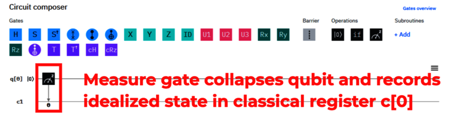
You can also directly declare a Measure gate in code by first specifying the gate, followed by the action the gate does on the qubit. In this case the Measure gate collapses the qubit in q[0] and logs the associated binary state to the classical register, c[0].
| | measure q[0] -> c[0]; |
This completes the quantum circuit for the Measure gate writing to a classical register. Here’s complete code listing:
| | OPENQASM 2.0; |
| | include "qelib1.inc"; |
| | qreg q[1]; |
| | creg c[1]; |
| | |
| | measure q[0] -> c[0]; |
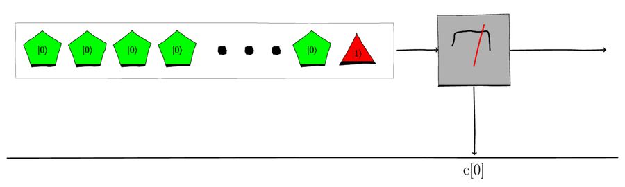
Since the qubit in the quantum register q[0]
is initialized to ![]() , the
quantum circuit effectively looks like the following
figure:
, the
quantum circuit effectively looks like the following
figure:

The qubelets in the box on the left simply
indicate the quantum state of
![]() —they’re not related to the
length of the quantum register array.
—they’re not related to the
length of the quantum register array.
When the Measure gate acts on the
q[0] qubit, it selects a random
qubelet from its quantum state, collapses it,
and writes the state of the selected qubit to the
classical register, c[0], as a binary bit.
Since the q[0] qubit is initialized
to ![]() , its quantum state
only has pentagon
, its quantum state
only has pentagon ![]() qubelets,
as shown in the previous figure. Thus, the
Measure gate always selects a
pentagon
qubelets,
as shown in the previous figure. Thus, the
Measure gate always selects a
pentagon ![]() qubelet and
writes a 0 to the classical register,
c[0].
qubelet and
writes a 0 to the classical register,
c[0].
Don’t Add Gates After a Measure Gate | |
|---|---|
|
|
Do not attach any gates to a qubit after you’ve measured its value with a Measure gate. Although the qubit is still active, its quantum state before you measured it is forever lost. In particular, don’t use them to debug your program, as you’ll get inconsistent or meaningless results. |
Running the Quantum Program
To run this quantum program, click the Run button on the top right of the window. (If the button is grayed out, Save your program first.) The dialog window shown opens.

Before running the program, you need to specify the following:
-
Select the quantum computer (the backend) you’d like to run your program on. The drop-down lists the available quantum computers that IBM offers, as well as a simulator.
The simulator will run your code immediately. The actual quantum computers run in the cloud—executing your code on one of them depends on the number of other programs in queue, so your program’s execution may be delayed.
-
As we discussed in Measure Gate, because the Measure gate randomly picks a qubelet from the quantum state of the qubit it’s acting on, all quantum programs are run multiple times. Each run is a shot. The goal of quantum computing, then, is to design algorithms that tilt the odds so that the optimal solution is returned in the vast majority of shots.
The results of your program’s execution will appear as a link in the Result section below the Composer. When you click the link, you will see the following Results page:
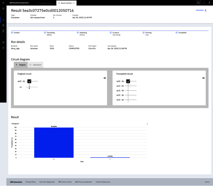
At the top of the page, the runtime metrics are listed. Next, you’ll see the following sections:
- Original Circuit:
-
This is the circuit you built on the Composer.
- Transpiled Circuit:
-
The circuit diagram you entered on the Composer is compiled, or transpiled, in which some gates are substituted with equivalent ones before your code is executed. We’ll see examples of these replacements in later chapters. For the most part, though, you don’t need to worry about this circuit.
- Result:
-
The results of your program’s execution appear in this section. A quantum program logs the results of its execution differently from how classical programs would. In a classical program, you have a wide variety of ways of documenting the results of a run, such as printing the values of your program’s variables when your code terminates. In quantum programming, the results of an execution are recorded in the classical registers as binary bits corresponding to the collapsed states of qubits. In other words, when your quantum program terminates, each classical register will hold a binary bit: 0 or 1. In particular, because a quantum program is run multiple times, the number of times each binary bit is seen in a register is shown as a percentage.
Running on a Simulator
If you elected to run your code on the simulator, the results of your run will be shown as follows:
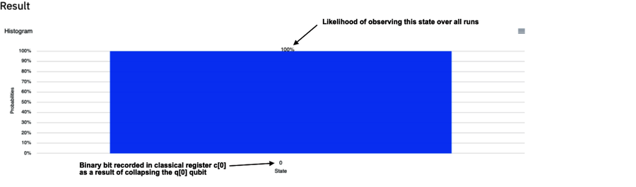
The value recorded in the classical register,
c[0], is shown at the base of the
big blue bar. The height of the big blue bar is
the confidence or probability of observing the
value shown at the base of the bar.
In the case of a ![]() qubit,
the computer’s confidence that it collapses
to
qubit,
the computer’s confidence that it collapses
to ![]() , corresponding
to the binary state 0, is 100%;
in other words, the probability
that c[0] = 0 is 1, an unequivocal
certainty.
, corresponding
to the binary state 0, is 100%;
in other words, the probability
that c[0] = 0 is 1, an unequivocal
certainty.
Running on a Real Quantum Computer
If, instead, you ran your program on a real quantum computer, your output will be similar to the following figure:

On a real quantum computer, in most shots
the Measure gate collapses the qubit to
![]() as expected. But in a small percentage of shots,
the qubit collapses to
as expected. But in a small percentage of shots,
the qubit collapses to ![]() .
So we see
two bars in the this figure: the taller bar is the
higher percentage for the classical register, c[0],
holding the corresponding binary bit, 0, and the
shorter one for the
classical register logging 1.
.
So we see
two bars in the this figure: the taller bar is the
higher percentage for the classical register, c[0],
holding the corresponding binary bit, 0, and the
shorter one for the
classical register logging 1.
The reason why we see a tiny fraction of shots
in which the Measure gate collapses
the ![]() qubit yet writes the binary
bit 1 to the classical register lies with the
way real qubits exist in nature.
qubit yet writes the binary
bit 1 to the classical register lies with the
way real qubits exist in nature.
Artificial qubits used in a simulator are
“pure.” That is, a ![]() qubit will have only pentagon
qubit will have only pentagon ![]() qubelets. Real qubits, on the other hand, are
not always precisely aligned
within the magnetic fields of the quantum computer’s
hardware. Conceptually, we model a real
qubelets. Real qubits, on the other hand, are
not always precisely aligned
within the magnetic fields of the quantum computer’s
hardware. Conceptually, we model a real
![]() qubit as follows:
qubit as follows:

The vast majority of qubelets in the real
![]() qubit are the pentagon baby
qubit are the pentagon baby
![]() qubelets.
But there’s also a smattering of
qubelets.
But there’s also a smattering of ![]() triangle qubelets.
triangle qubelets.
Likewise, a “real” ![]() qubit is shown as follows:
qubit is shown as follows:

So when we’re working with real qubits, our quantum circuit looks like the following figure:
When the Measure gate collapses the
real ![]() qubit
on the left, there’s a small chance that a
triangle
qubit
on the left, there’s a small chance that a
triangle ![]() gets selected.
Thus, a binary 1 bit is written
in the classical registers on those seldom occasions.
Consequently, every now and then, you’ll
see this errant behavior show up as tiny bars on
the output graph.
gets selected.
Thus, a binary 1 bit is written
in the classical registers on those seldom occasions.
Consequently, every now and then, you’ll
see this errant behavior show up as tiny bars on
the output graph.
As the engineering of quantum computers improves, the effect of noise will reduce. So we won’t worry about the difference between real and artificial qubits in our quantum programs. But when interpreting the outputs of your programs, you’ll sometimes see them collapsing the qubits incorrectly. Discard these states as noise.