Programming with Qiskit

Although we’ve used the QASM language to program our quantum circuits on the IBM Quantum Computer, the primary way we coded the circuits was by dragging and dropping gates from the gates palette onto the Composer. This drag-and-drop process results in the circuits being programmed in the QASM language.

But QASM is a low-level assembly language that we can’t integrate with other systems, such as a database to pull in data to build circuits. Dragging and dropping gates lets us learn about quantum concepts without getting distracted by classical language-specific constructs. In practice, though, you’ll want to invoke quantum phenomena in conventional programming languages. In this section, you’ll learn to incorporate quantum effects in classical languages. You’ll still design quantum algorithms using the techniques you’ve learned in this book, but you’ll use classical languages to program and execute them on real quantum computers.

Quantum Information Science Kit, or Qiskit (pronounced kiss-kit), is a Python framework that IBM has contributed to the open source community. Using Qiskit,^[76] you can use all the quantum effects you’ve learned in this book but program them in Python, although the code is executed on the IBM Quantum Computer or a simulator. While the drag-and-drop way of programming quantum computers is good when learning about quantum concepts, Qiskit comes packed with goodies that let you write industrial-grade quantum code. I’ll first introduce you to the basics of using Qiskit and then show you things you can do only with it.

Quantum Programming Is Not Python Specific

With Qiskit, you’ll program quantum effects using Python, but quantum computing isn’t Python specific. Quantum concepts are independent of any language. You’ll still design quantum algorithms using the techniques you’ve learned in this book—Qiskit is an alternative way to trigger them on IBM’s quantum hardware, using Python instead of the QASM assembly language. Later in this section, you’ll see that these same quantum effects can be triggered on quantum hardware of other vendors, such as Amazon, Google, and Microsoft. To use the programs in this section, you should, nonetheless, know Python,[77] [78] including working with arrays and complex numbers and opening and navigating your way in Jupyter Notebooks[79] on your local machine.

You can use Qiskit in one of two ways:

• On the IBM Quantum Experience website, using Jupyter Notebooks.
• Locally on your machine by writing Python programs or coding in Jupyter Notebooks.

We’ll briefly go over getting started with both ways. Then you can choose whichever mode you prefer to program with Qiskit.

Using the IBM Quantum Experience

To use Qiskit on the IBM Quantum Experience, you can click the Qiskit Notebook icon on the left margin, as shown in the following figure:

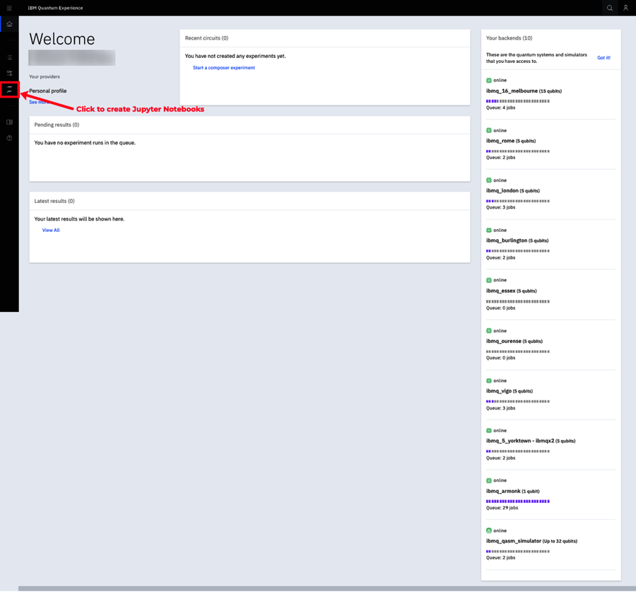
You’ll be taken to a page where you can create a new Jupyter Notebook or open one that you created previously.

On the IBM Quantum Experience, new notebooks have the statements to import the Qiskit libraries as well as configure the notebook to access the methods to run on a real quantum computer. For now, you can delete these lines. I’ll show you what you need to import to run the programs in this section. (If you choose to leave them in, then make sure you include any specific ones I highlight in the programs.)

Working Locally

To work in Jupyter Notebooks locally, first install Qiskit on your computer, from here,^{[80] [81]} and follow the instructions for your operating system. Note that to run Qiskit, Python 3 is required.

To make sure you’ve installed Qiskit correctly, you can check its version by opening a new Python 3 Jupyter Notebook and typing in the following lines in a code cell. Then hit Shift-Enter to execute them:

​	​import​ ​qiskit​
​	​from​ ​qiskit​ ​import​ *
​
​	qiskit.__qiskit_version__

You’ll see a list of the various components that make up Qiskit and their respective versions.

Now you’re ready to write your first quantum program with Qiskit.

Jupyter Notebooks
	We’ll use Python 3 Jupyter Notebooks in this section so they can be used interchangeably on both the IBM Quantum Experience and on your local machine.

Hello Qiskit

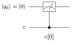
To get started with Qiskit, consider the following quantum circuit that has just a single qubit which is immediately collapsed by the Measure gate shown in the figure.

The Python code for this circuit follows the same general structure of the programs written earlier but also includes the instructions to execute the circuit on quantum hardware:

• Declare quantum and classical registers to hold the qubits and their collapsed states, respectively.

• Declare the quantum gates that act on the qubits.

• Collapse the qubits using the Measure gates, and log their states in the classical register.

• Specify how many shots, or the number of times you want to run the circuit.

• Run the circuit.

• View the results.

These general steps translate to the following Python code:

​​①​	​import​ ​numpy​ ​as​ ​np​
​	​import​ ​math​
​	​from​ ​qiskit​ ​import​(
​	QuantumCircuit,
​	QuantumRegister,
​	ClassicalRegister,
​	execute,
​	Aer)
​	​from​ ​qiskit.visualization​ ​import​ plot_histogram
​
​​②​	circuit = QuantumCircuit()
​
​​③​	q = QuantumRegister(1,​'qreg'​)
​	circuit.add_register( q )
​
​​④​	c = ClassicalRegister(1,​'creg'​)
​	circuit.add_register(c)
​
​​⑤​	circuit.measure(0,0)
​
​​⑥​	circuit.draw(output=​'mpl'​)
​
​​⑦​	backend = Aer.get_backend(​'qasm_simulator'​)
​
​​⑧​	job = execute( circuit, backend, shots=1024 )
​
​​⑨​	hist = job.result().get_counts()
​	plot_histogram( hist )

​①​

The NumPy library will let you handle arrays of qubits in your applications. The math library lets you use mathematical functions in your programs. To use Qiskit, you need to import the Qiskit libraries. The other libraries are related to the Qiskit objects you’ll use in your programs. As you get more familiar with Qiskit, you’ll understand which ones you’ll need. For now, you can just copy and paste these.

​②​

Define a circuit object to which gates will be added.

​③​

Declare and add the quantum register to hold the qubits in the circuit.

The first argument is the length of the register and the second is its label. In this case, there’s only a single qubit in the circuit. All qubits are initialized to .

​④​

Declare and add the classical register to record the collapsed states of the qubits in the circuit.

The first argument is the length of the register and the second is its label. In this case, there’s only a cell to record the solitary qubit in the circuit.

​⑤​

Declare the Measure gate. The first argument is the index of the qubit in the quantum register you want to collapse; the second is the index in the classical register where you want to log the state. For this circuit, the collapsed state of q[0] is recorded in c[0].

​⑥​

This command draws the quantum circuit. When working in Jupyter Notebooks, you may want to periodically draw the circuit as you’re building it to make sure it’s correct.

The argument refers to the style of the circuit layout. The mpl option uses Python’s Matplotlib visualization library to draw the circuit that closely resembles the circuits on the Composer. Leaving this argument blank uses the default library on the machine where your notebook is executing. On the IBM Quantum Experience, the default option is mpl. So you can invoke the draw method with no arguments.

​⑦​

Identify the quantum machine, or backend you want this code to run on. In this case, we’re using the qasm_simulator, which isdefined in the Aer object, to run the circuit.

Aer^[82] is Qiskit’s simulator framework that lets you simulate the noisy behavior of real quantum devices. In addition, using the statevector_simulator, it calculates the Statevector of the circuit and, with the unitary_backend, the matrix for the complete circuit.

​⑧​

Run the code on the selected backend or quantum machine. You pass the quantum circuit in the first argument, specify the backend in the second, and the number of shots in the third.

​⑨​

Tally up the number of times each quantum state the qubits collapse to and plot as a histogram.

Pasting Code in Jupyter Notebooks

Before pasting code into Jupyter Notebooks, make sure you’ve imported the Qiskit and relevant Python libraries, such as NumPy and math: ​  ​from​ ​qiskit​ ​import​( ​  QuantumCircuit, ​  QuantumRegister, ​  ClassicalRegister, ​  execute, ​  Aer) ​  ​from​ ​qiskit.visualization​ ​import​ plot_histogram You can directly copy and paste the code you’ll see in this chapter into Python 3 Jupyter Notebooks. You can paste into a single code cell or split it across as many cells as you’d like. To run the code in a code cell, click Shift-Enter. Be aware that the code you enter is cumulative. That is, any new gates you declare are added to the circuit previously defined. Thus, you may end up with a circuit that you didn’t intend.

You’ll follow this basic structure to declare and run other quantum circuits on quantum computers—you’ll just have more gates.

Quantum Gates in Qiskit

In Qiskit, each gate is a method of the circuit object. Thus, to declare a gate, you’d invoke the appropriate method followed by the qubits it operates on as arguments for the method. The following is a partial list to show you the general pattern for declaring gates in your circuit:

H Gate:

To use an H gate acting on the qubit in register q[0], declare it as follows:

​	circuit.h( q[0] )

S Gate:

To use an S gate acting on, for example, the qubit in register q[1], declare it as follows:

​	circuit.s(q[1])

Gate

To use a gate acting on, for instance, the qubit in register q[2], declare it as follows:

​	circuit.tdg(q[2])

Notice how the “dagger” symbol is abbreviated to “dg” when declaring these types of gates.

CNOT Gate

To use a CNOT gate whose control bit is, for example, the qubit in register q[3] and whose target qubit is in register q[4], declare is as follows:

​	circuit.cnot(q[3],q[4])

U3 Gate

To use a U3 gate that’s defined using three parameters, , , and , which operates on, say, the qubit in q[3], declare it as follows:

​	circuit.u3(0,math.pi,0,q[3])

Here, the U3 gate’s parameters are set to , , and . (Recall from ​U3 Gate​, that these parameters only affect the triangle qubelet by inverting it, or rotating it by half a turn.)

Measure Gate

To measure, for instance, the qubit in register q[0] and record its state in classical register c[0], declare it as follows:

​	circuit.measure(q[0],c[0])

The first argument refers to the qubit, and its collapsed state is logged in the classical register in the second argument.

To use these gates, you should have previously declared the circuit object as, for example, circuit = QuantumCircuit() and also the qubits as q = QuantumRegister(5,’qreg’), a quantum register holding five qubits, followed by circuit.add_register(q) to add the qubits to the circuit.

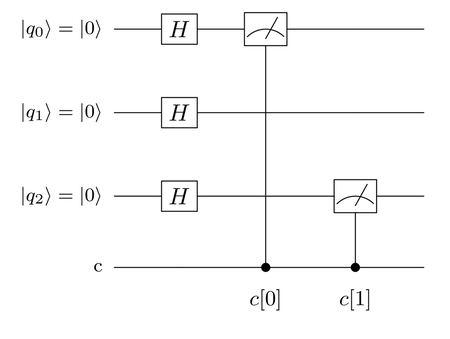
Consider, again, the Qiskit program for the quantum circuit in ​Intuition Behind Entanglement​, shown in the figure.

The Qiskit program is listed here:

​1:	​# Header lines - import libraries​
​-	​import​ ​numpy​ ​as​ ​np​
​-	​import​ ​math​
​-	​from​ ​qiskit​ ​import​(
​5:	QuantumCircuit,
​-	QuantumRegister,
​-	ClassicalRegister,
​-	execute,
​-	Aer)
​10:	​from​ ​qiskit.visualization​ ​import​ plot_histogram
​-
​-	​# Define circuit​
​-	circuit = QuantumCircuit()
​-
​15:	​# Declare and add quantum and classical registers​
​-	q = QuantumRegister(2,​'qreg'​) ​# 2 Qubits Register​
​-	circuit.add_register( q )
​-
​-	c = ClassicalRegister(2,​'creg'​) ​# 2 Bits Classical Register​
​20:	circuit.add_register(c)
​-
​-	​# Declare the H Gate​
​-	circuit.h(q[0])
​-
​25:	​# Declare the CNOT Gate​
​-	circuit.cnot(q[0],q[1])
​-
​-	​# Collapse Qubits​
​-	circuit.measure(q[0],c[0])
​30:	circuit.measure(q[1],c[1])
​-
​-	​# Draw the circuit​
​-	circuit.draw(output=​'mpl'​)
​-
​35:	​# Use simulator to run the circuit​
​-	backend = Aer.get_backend(​'qasm_simulator'​)
​-
​-	​# Define the run parameters and execute​
​-	job = execute( circuit, backend, shots=1024 )
​40:
​-	​# Tally the results​
​-	hist = job.result().get_counts()
​-
​-	​# Plot the histogram of quantum states​
​45:	plot_histogram( hist )

The H, CNOT, and the two Measure gates are declared on lines 23--30. The rest of the program is similar to that listed previously.

When you run this program, you’ll see the output states, and , appear with roughly equal probabilities. (These states are entangled because once you observe one, the other’s state is known even if the other qubit isn’t measured.)

Qiskit Shortcuts

If you’re not picky about labeling your quantum and classical registers and can work with a single register of each, you can declare quantum circuits and the gates as follows:

Declaring Circuit and Quantum Register

You can declare the QuantumCircuit object and the quantum register by passing in the length of register, or the number of qubits in the circuit, as an argument to the QuantumCircuit object as follows:

​	circuit1 = QuantumCircuit(5)

This statement declares a circuit with five qubits.

Declaring Circuit with Both Quantum and Classical Registers

To set up a circuit with both quantum and classical registers, pass the length of both registers, respectively, as follows:

​	circuit2 = QuantumCircuit(3,2)

The first argument is the number of qubits in the circuit, and the second is the number of bits in the classical register. In this case, the circuit has three qubits and two bits in the classical register.

Declaring Gates

To declare gates and the qubits they act on, you can specify just the index of the qubit in the quantum register. For example, to declare an H gate that operates on, say, the qubit in q[2], declare it as follows:

​	circuit1.h(2)

Arrays as Arguments

Qiskit also lets you pass in arrays as arguments for the gates to create multiple gates. To create an H gate on all four qubits of circuit2 defined earlier, pass the array of qubits, using Python’s built-in range function, for instance, as follows:

​	circuit2.h(range(3))

You can even pass in arrays as arguments for the Measure gate. For example, you can declare Measure gates on qubits q[0] and q[2] that log their states in the classical register cells c[0] and c[1], as follows:

​	circuit2.measure([0,2],[0,1])

The previous two statements set up the following quantum circuit:

Running on an Actual Quantum Computer

Running your programs on an actual quantum computer follows the same basic steps as that of using the simulator, except for a few minor differences, which I’ll discuss in this section:

API Token:

Include the API token in your code, which lets you execute your programs on an actual quantum computer.

Backend to Run Code:

Replace the code to run on the simulator with one of the actual quantum computers.

Viewing the Results:

Because running code on a quantum computer doesn’t take place immediately, due to other programs ahead of yours, you have to break up your program into two parts: one to set up the quantum circuit and invoke the quantum computer and the second to view the results of your run later.

Saving the API Token for Working Locally

If you’d like to run your Qiskit programs on a real quantum computer but trigger it locally, you need to first save an API token on your local machine.^[83] (When running Jupyter Notebooks from your account on the IBM Quantum Experience, you don’t need to save it. You only need to include it, as shown in the following description.)

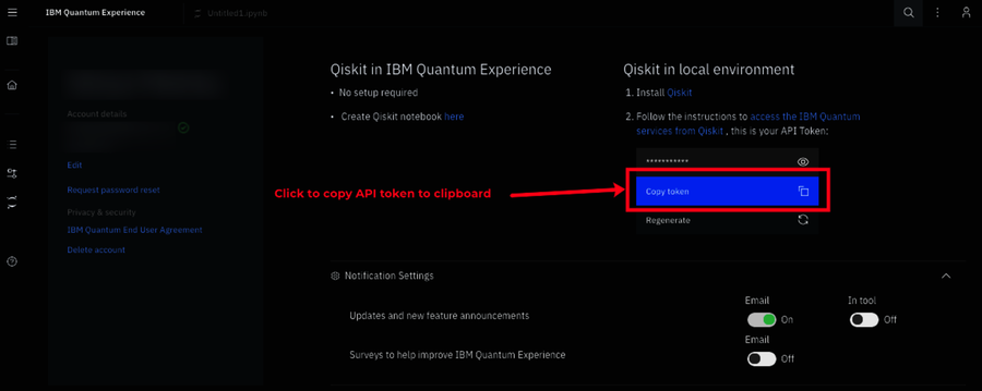
The API token is listed under your account information on the home page of the IBM Quantum Experience. To get the API token, go to your user profile by either clicking the See more link or the user icon on the top right, as shown in the following figure:

Then, click the Copy token link as shown in the figure.

Next, on your local machine, open a new Jupyter Notebook, type in the following lines, and paste the API token as shown:

​	​from​ ​qiskit​ ​import​ IBMQ
​
​	IBMQ.save_account(​'API Token'​)

To save the API token to your machine, execute the cell by pressing Shift-Enter. You only need to save it once.

If you have an API token from a version of Qiskit older than 0.11, update your token as follows:

​	IBMQ.update_account()

Backend to Run Code

To set up your quantum circuit to run on a real quantum computer, you follow the same steps to define your quantum circuit. But instead of selecting the simulator, pick one of the real quantum computers, as shown here:

​	​from​ ​qiskit​ ​import​(
​	QuantumCircuit,
​	QuantumRegister,
​	ClassicalRegister,
​	execute,
​	Aer,
​​①​	IBMQ)
​​②​	​from​ ​qiskit.providers.ibmq​ ​import​ least_busy
​	​from​ ​qiskit.visualization​ ​import​ plot_histogram
​
​​③​	provider = IBMQ.load_account()
​
​	Set up Quantum Circuit
​
​​④​	real_devices = provider.backends(simulator=False, operational=True)
​	backend = least_busy(real_devices)
​
​​⑤​	job = execute( circuit, backend, shots=1024 )

​①​

Import Qiskit, including the IBMQ library, to access the methods to run on a real quantum computer. Also, import the least_busy library to identify the real quantum computer with the lightest load.

​②​

To run your code on the quantum computer that has the fewest jobs in queue, select the least busy backend.

​③​

Define a provider object by loading it with the saved API token. You’ll need this when running Jupyter Notebooks on the IBM Quantum Experience or locally.

​④​

Filter the list of available backends to those that are real quantum computers and currently operational. From this list, select the one that has the fewest number of jobs.

​⑤​

Just as with the simulator, run your program with the backend selected in the previous step. Depending on the number of jobs ahead of yours, you may have to come back later to view the results.

To run your program on a specific quantum computer, get the list of available backends:

​	provider.backends()

Then, use the get_backend method on the provider object and pass in the name of the quantum computer, as follows:

​	backend = provider.get_backend(​'ibmq_16_melbourne'​)

In this case, we’ve selected the 16-qubit quantum computer in Melbourne. Execute your circuit on this backend.

To learn about other things you can do with the provider object, go here.^[84]

Viewing the Results

To view the results of running your program on a real quantum computer, get the Job ID of the execution from the IBM Quantum Experience website, as shown in the figure.

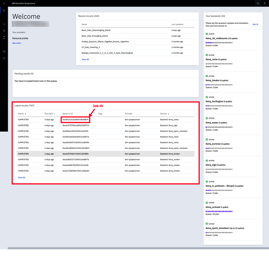
Copy the Job ID onto the clipboard.

Unless you’ve left your notebook running, open a new notebook, import the standard Qiskit libraries, and define a provider object with your API token. Then, specify the backend on which you ran your code and paste the Job ID, as shown next:

​	provider = IBMQ.load_account()
​	backend = provider.get_backend(​'Backend'​)
​	job = backend.retrieve_job(​'Job ID'​)

This gets the job object, just as when you ran a quantum program on the simulator. Access the results and tally them up by how many times each state is logged. Finally, plot the counts as a histogram chart, shown as follows:

​	hist = job.result().get_counts()
​	plot_histogram( hist )

Now that you’ve seen how to build and run your quantum programs on a simulator as well as on real quantum hardware—including using shortcuts to declare mulitple gates in a single statement—in the rest of this section, you’ll see a few features that you can only use with Qiskit and not in the drag-and-drop programs created with the IBM Quantum Experience.

Creating Larger Circuits from Smaller Circuits

As your programs get larger, you’ll find it helpful to write modular code. That is, you’ll want to define chunks or groups of gates that you can use in many places in your circuit as a unit without having to individually insert the gates that make up the block. You can do this two ways:

User-Defined Gates:

Create groups of gates that collectively perform some operation such as swapping the quantum states of two qubits, or the Boolean logic operations such as OR.

Partial Circuits:

Create partial circuits that you can then hook up to make a larger circuit. For example, you make a partial circuit that generates all combinations of quantum states. You can then plug this circuit into another one that, say, implements Boolean logic expressions.

User-Defined Gates

Qiskit lets you group gates and then refer to them as a single unit in your circuit. To specify these user-defined gates,^[85] follow these steps:

• Define the configuration of gates as a circuit object, as explained earlier.
• Make these gates an instruction.
• To use it in your circuit as a single unit, Append it to the main circuit object.

Consider, for example, an OR gate, defined in ​OR Gate​, and shown in the figure below:

To define this configuration of the CCNOT gate and the associated NOT (X) gates as an or_gate gate in your Python code, start by setting up these gates as an or_gate_circuit object:

​1:	or_gate_circuit = QuantumCircuit(3, name=​' OR '​)
​2:	or_gate_circuit.x(range(3))
​3:	or_gate_circuit.ccx(0,1,2)
​4:	or_gate_circuit.x(range(2))
​5:	or_gate = or_gate_circuit.to_instruction()

Declare the circuit object for the OR gate with three qubits, as shown on line 1. The name parameter is the label for this group of gates when the circuit is displayed. Notice how we’ve padded the label with a space on either side of the text. This puts some margin on either side of the label in the box for the gate when it’s shown in the circuit.

If you don’t plan on viewing the circuit, you can leave it blank; the system will assign a generic label.

Declare the gates that make up the OR gate on lines 2--4. Notice how the X gates are declared by passing in the appropriate array as the argument. For example, to create the two NOT (X) gates on the right, the argument for the NOT (X) gate on line 4 is an array formed by range(2).

The way we’ve set up the OR gate implies that the input qubits are in q[0] and q[1] and the result of the logical OR operation is reflected in the qubit in q[3]. The order of the qubits—q[0], q[1], and q[2]—define the arguments for this group of gates.

Finally, on line 5, convert this group of gates to an Instruction so that it can be inserted in the main circuit as just another gate.

For example, look at a circuit in which the OR gate is hooked up as follows:

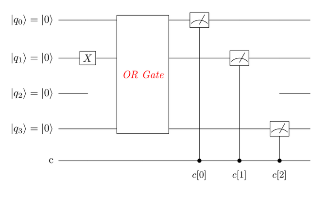
The OR gate operates on the qubits in q[0] and q[1] and puts the results of the operation in the qubit in q[3]. Since the qubit in q[1] is first acted on by the NOT (X) gate, its state is changed to .

The Qiskit code for this circuit is as follows:

​1:	main_circuit = QuantumCircuit(4,3)
​2:	main_circuit.x(1)
​3:	main_circuit.append(or_gate, [0,1,3])
​4:	main_circuit.measure([0,1,3],[0,1,2])

On line 1, declare the main_circuit using four qubits and three classical registers. On line 2, set the qubit in q[1] to with an NOT (X) gate. On line 3, add the OR gate you configured previously to the main_circuit. The first argument is the circuit object for the group of gates for the OR gate. The qubits in q[0] and q[1] are the inputs, and the qubit in q[3] holds the result of the logical OR operations. This set of qubits is passed in as an array as the second argument of the append method. Lastly, on line 4 declare the Measure gates. The qubits being measured, q[0], q[1], and q[3], are passed in as array in the first argument. And the classical registers that log their collapsed states are also passed in as an array in the second argument to the Measure gate’s method.

If you’d like to see the OR Gate block replaced with the actual gates that make it up, use the decompose method of the circuit object, as follows:

​	decomposed_circuit = main_circuit.decompose()

You’ll see the following circuit:

The dashed box is only to illustrate to you the new gates shown. It’s not drawn by Qiskit. Notice that even though the target qubit of the CNOT gate was specified right below its second control qubit, in the actual circuit it’s two qubits below, as was defined in the second argument of the append.

Partial Circuits

Qiskit lets you break up your circuits into functional units and build each separately. Then, you can simply hook them up one after another by “adding” them. The circuits should have the same number of qubits.

For example, consider the following circuit that generates all combinations of three qubit states:

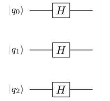
You can set these gates in an all_combinations_circuit as follows:

​	all_combinations_circuit = QuantumCircuit(3)
​	all_combinations_circuit.h(range(3))

Likewise, you can set up a measure_circuit that has the same number of qubits but only two classical registers:

​	measure_circuit = QuantumCircuit(3,2)

And you can define the Measure gates to record the states of qubits in q[0] and q[2] as follows:

​	measure_circuit.measure([0,2],[0,1])

The quantum state of the qubit in q[0] is logged to c[0] and that of the qubit in q[2] to c[1].

Now, “add” the two circuits, stated as follows:

​	new_circuit = all_combinations_circuit + measure_circuit

This creates the following circuit:

Output States as an Array

In all the quantum programs you’ve seen in this book, the output is reported as a histogram of quantum states. When writing applications for real world problems, though, you may want the results in a form that you can do some further processing on.

After executing the circuit, the metrics for that run are held in the Result object. Use the get_counts to pull out the tallies of each of the idealized states as an array, shown as follows:

​	Import Qiskt, other libraries
​	Set up Quantum Circuit
​
​	​# Use simulator to run the circuit​
​	backend = Aer.get_backend(​'qasm_simulator'​)
​
​	​# Define the run parameters and execute​
​	job = execute( circuit, backend, shots=1024 )
​
​	​# Tally the results​
»	collapsed_states_array = job.result().get_counts()
​	​print​(collapsed_states_array)

The system will return a dictionary of name-value pairs, as shown here:

​	{​'01'​: 520, ​'10'​: 504}

Each name-value entry corresponds to an idealized state. The name is the state and the value is the number of times that state was seen in the execution. In this example, the 01 state appeared 520 times out of 1,024 shots.

You can now extract these states and their counts from the array and use them in your application.

Displaying the Statevector

To display the Statevector, the quantum state vector, you have to use the statevector_simulator backend, shown as follows:

​	Import Qiskt, other libraries
​	Set up Quantum Circuit
​
»	backend = Aer.get_backend(​'statevector_simulator'​)
​	job = execute(circuit, backend)
​	result = job.result()
»	statevector = result.get_statevector(decimals=3)
​	​print​(statevector)

Then, as highlighted in the code, use the get_statevector method on the result object to get the quantum state as a Python array.

For example, consider the quantum state :

The corresponding vector is:

Qiskit would return this vector as the following Python array where each entry is written up to three decimal places:

​	[0. +0.j 0.707+0.j 0.707+0.j 0. +0.j]

Each element is stated as a complex number using instead of (both are mathematically equivalent).

Circuit Matrices

Qiskit also gives you the matrix for your quantum circuit. To get this matrix, you have to run your circuit on the unitary_simulator backend, as the following shows:

​	Import Qiskt, other libraries
​	Set up Quantum Circuit
​
​	​# Run the quantum circuit on a unitary simulator backend​
»	backend = Aer.get_backend(​'unitary_simulator'​)
​	job = execute(circuit, backend)
​	result = job.result()
​
​	​# Show the results​
»	​print​(result.get_unitary(circuit, decimals=3))

Then, as highlighted in the code, use the get_unitary method on the result object to get the matrix of the circuit as an “array of arrays.”

Setting Up Arbitrary Quantum States

In all the circuits you’ve seen so far, the qubits are initialized to . Qiskit gives you a mechanism to initialize the amplitudes^[86] of the idealized states to any value provided the respective probabilites—square of the amplitudes—add up to 1.

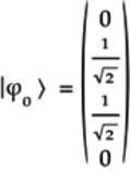
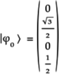
For example, suppose you want to set the initial quantum state of a two-qubit system to:

Writing as a vector:

Remember that when programming the IBM Quantum Computer, the rightmost bit refers to . Thus, the quantum state is actually the state for the IBM Quantum Computer. Hence, the second element is in the quantum state vector stated above. The first and third elements are 0 as they correspond to states that are not present in the initial quantum state.

Set up this vector in Python as an array labeled input_quantum_state:

​	Import Qiskt, math, NumPy libraries
​
​	​# Define the input quantum state​
​	input_quantum_state = [0,
​	math.sqrt(3)/2*complex(1,0),
​	0,
​	1/2 * complex(1,0)]

The array has the four elements corresponding to the vector .

Next, initialize the quantum circuit with this quantum state, as follows:

​1:	​# Initialize circuit​
​2:	q = QuantumRegister(2)
​3:	c = ClassicalRegister(2)
​4:	circuit = QuantumCircuit(q,c)
​5:	circuit.initialize(input_quantum_state, q)

Set up a two-qubit quantum circuit with two classical registers on lines 2--4. Initialize the circuit on line 5 with the initialize method that takes in two arguments: the initial quantum state vector and the quantum register array q.

You can check that the circuit is indeed initialized with this quantum state by looking at its Statevector:

​	backend = Aer.get_backend(​'statevector_simulator'​)
​	job = execute(circuit, backend)
​	result = job.result()
​	statevector = result.get_statevector(decimals=3)
​	​print​(statevector)

Running these lines returns the following array:

​	[0. +0.j 0.866+0.j 0. +0.j 0.5 +0.j]

This array corresponds to the quantum state vector .

Gates from Matrices

In Chapter 7, ​Small Step for Man—Single Qubit Programs​, you learned that when quantum states are represented by vectors, the operation of a gate can be modeled by matrices. Using Qiskit you can go the other way. When designing quantum algorithms, you know the way you want to manipulate quantum states. With Qiskit, you can define the corresponding matrix, and the system generates the implied circuit internally. Think of this feature as a many-qubits Universal gate.

The matrix you define must be unitary, as explained in ​Can the Quantum Gate Matrix Be Anything?​.

To use these user-defined matrices in your code, do the following:

Import the Operator Library:

To use your matrix as a gate in your code, import the library shown in the highlighted line in the following:

​	​import​ ​numpy​ ​as​ ​np​
​	​import​ ​math​
​	​from​ ​qiskit​ ​import​(
​	QuantumCircuit,
​	QuantumRegister,
​	ClassicalRegister,
​	execute,
​	Aer)
​	​from​ ​qiskit.visualization​ ​import​ plot_histogram
»	​from​ ​qiskit.quantum_info.operators​ ​import​ Operator

Define the Gate Matrix:

The matrix is defined as a standard Python list of lists: each row of the matrix is a list. For example, consider the matrix for a two-qubit gate defined as follows:

This matrix is represented as a list of lists and passed in as the argument to the Operator method, shown as follows:

​	my_gate_2 = Operator([
​	[math.sqrt(3)/2, 0, 1/2, 0],
​	[0, math.sqrt(3)/2, 0, 1/2],
​	[1/2*complex(0,1), 0, -math.sqrt(3)/2*complex(0,1),0],
​	[0,1/2*complex(0,1),0, -math.sqrt(3)/2*complex(0,1)]
​	])

Define Matrices Using IBM’s Convention for Writing Quantum States

When specifying the matrix for the gate in Qiskit, define the matrix using IBM’s convention for writing the quantum state with the q[0] qubit in the least significant place or in the rightmost spot. For example, would actually be written as 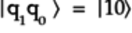when specifying the matrix in Qiskit. To put it another way, the second column, say, in a matrix for a two-qubit gate will still correspond to the state but is defined as . So when working out the matrix, make sure you’re correctly lining up the quantum states in your circuit so that the state in qubit q[0] is in the rightmost spot, and so on.

Before using this gate in your code, it’s a good idea to check whether it’s unitary by calling the is_unitary method, as follows:

​	​# Check unitary​
​	​print​(​'Operatator is unitary:'​, my_gate_2.is_unitary())

If it’s not unitary, fix the matrix; otherwise, you’ll get errors when trying to run your program.

Using the Matrix in a Circuit:

To use this matrix in a circuit, use the append on the circuit object passing in the matrix as the first argument and the array of qubits the gate acts on in your circuit as the second argument, shown here:

​	circuit.append(my_gate_2, [0,1])

In this case, the first qubit that the two-qubit gate acts on is q[0] and the second is q[1].

Qiskit offers a rich set of functions for matrix operations, such as computing their tensor products. You can find more information here.^[87]

Circuit Metrics

Qiskit’s circuit object has several attributes and properties that give you information and metrics about your circuit.^[88] We’ll use the following circuit as a reference:

Here’s the Qiskit code to set up this circuit:

​	Import Qiskt, math, NumPy libraries
​	circuit = QuantumCircuit(3,2)
​	circuit.h([0,2])
​	circuit.s(2)
​	circuit.cx(0,1)
​	circuit.measure([0,2],[0,1])

Following is a list of some of this circuit’s metrics (all metrics are either attributes or methods of the circuit object):

Number of Quantum Registers

To get the number of quantum registers, look at the qregs attribute:

​	circuit.qregs

For the previous circuit, this number is the following:

​	[QuantumRegister(3, ​'q'​)]

The first argument is the number of quantum registers.

You can also directly get the number of qubits with the n_qubits attribute:

​	circuit.n_qubits

Number of Classical Registers

To get the number of classical registers, look at the cregs attribute:

​	circuit.cregs

For the previous circuit, this number is the following:

​	[ClassicalRegister(2, ​'c'​)]

Width or the Number of Quantum and Classical Bits

The width of a quantum circuit refers to the number of quantum bits as well as the number of classical bits making up the classical register. To get this count, use the width method:

​	circuit.width()

Having three qubits and a two-bit classical register, the width of this circuit is 5.

Number of Gates by Type

Qiskit can also tally up the number of gates of each type in a circuit by using the count_ops method, or the number of operations on qubits by the gates:

​	circuit.count_ops()

For the previous circuit, this works out to the following:

​	OrderedDict([(​'h'​, 2), (​'measure'​, 2), (​'s'​, 1), (​'cx'​, 1)])

You get an ordered dictionary in which each element’s key is the gate and value is the number of gates of that type. For example, the first element, (’h’,2) indicates that the previous circuit has two H gates.

Number of Operations

To get a count of the total number of operations on qubits by all gates in the circuit, use the size:

​	circuit.size()

For the previous circuit, the there are six operations: two for the H gates, two for the Measure, one for the S, and one for the CNOT gate. Notice that even though the CNOT gate acts on two qubits, it’s counted as a single operation, as it operates on them as a unit.

Depth or the Number of Simultaneous Operations

Generally speaking, a vertical slice through any circuit shows you the gates that can operate simultaneously on the qubits. Consequently, the number of these vertical slices translates to the amount of time a quantum program takes to run. The number of vertical slices, or layers, is called the depth of the quantum circuit.

Consider, again the quantum circuit shown earlier but, this time, with dotted boxes around the gates, representing the vertical slices, as shown in the following circuit:

Looking at these vertical slices, it seems that it has six layers. But you can “squeeze” some layers together, making the gates in them operate on the qubits at the same time without affecting the overall working of the circuit. That is, the circuit shown previously can be squeezed to that shown in the following figure:

This circuit has only three layers.

Qiskit can figure this out for your circuit by using the depth method, as stated here:

​	circuit.depth()

Number of Independent Sets of Qubits

The quantum circuit shown in the beginning of this section has three qubits—that is, its mega-qubit will have three cells in each qubelet combination. But, while the first two qubits, q[0] and q[1], are tightly coupled, or entangled, by the CNOT gate, the third qubit, q[2], is on its own. In other words, from a computational standpoint, you could technically first run the circuit with only the first two qubits and then combine the result with that of the run from the circuit with the third qubit. That is, this circuit has two independent sets of qubits: (q[0],q[1]), and (q[2]).

Using the num_unitary_factors method, Qiskit will return the number of independent sets of qubits:

​	circuit.num_unitary_factors()

More Commands

We’ve just mentioned a tiny fraction of Qiskit’s vast and rich features. Its documentation is comprehensive and easy to explore. By poking around, you’ll come across other features that may interest you, such as displaying the outputs of several runs side by side,^[89] showing the qubit on the Bloch sphere,^[90] and seeing amplitudes in 3D.^[91] Qiskit also lets you simulate the decoherence, or noise, of actual quantum computers in your simulations.^[92]