Grover’s Algorithm
Giving developers a way to simultaneously hold all
solutions to a problem is like taking kids to a candy
store but then having them first figure out the combination
of the lock to the store before they can eat all the
sweets they want. Likewise, quantum
computers exploit the natural ability of subatomic particles
to remain suspended so that each can collapse to
one of two states—a collection of ![]() quantum
particles effectively holds all 2n
states. But the challenge is to figure out how
to collapse the qubits so that they land on the
correct solution of the problem.
quantum
particles effectively holds all 2n
states. But the challenge is to figure out how
to collapse the qubits so that they land on the
correct solution of the problem.
When the constraints of the problem are well defined,
we can use Grover’s algorithm,[62] [63] a technique that identifies the optimal
solution from the mega-qubit by eliminating the non-optimal
ones.
(Also see Quantum Computer Science [Mer07].)
To use this algorithm, your application’s constraints must
be set up with Boolean logic expressions,
using the quantum logic gates as shown in
Logic Expressions to Quantum Circuit.
Think of these gates as a referee: given a potential solution
of ![]() and
and ![]() qubits, they’ll say whether the qubits satisfy the
Boolean logic expressions. For those
qubit values that meet the constraints, their qubelets
are rotated, or tagged, to distinguish
them from those that aren’t feasible.
The quantum logic gates don’t actually produce
a valid set of qubit values that satisfy the Boolean
logic expressions.
qubits, they’ll say whether the qubits satisfy the
Boolean logic expressions. For those
qubit values that meet the constraints, their qubelets
are rotated, or tagged, to distinguish
them from those that aren’t feasible.
The quantum logic gates don’t actually produce
a valid set of qubit values that satisfy the Boolean
logic expressions.
The quantum logic gates model the Boolean logic expressions we set up when we defined the problem. The solution we’re looking for is one that satisfies those expressions. A classical computer would test each solution in turn. The quantum circuit considers all the possible solutions in the mega-qubit at the same time, and the logic gates are used to eliminate all the solutions except for the correct ones. These steps are shown schematically in the following figure:
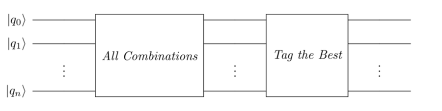
The high-level steps in Grover’s algorithm are shown by the following figure:

Tagging and Canceling Are Referenced Differently in the Literature | |
|---|---|
|
|
In the literature, the tagging phase is called the oracle—a function that decrees whether a given state of 0s and 1s qualifies as a solution for the Boolean logic expressions. The canceling phase is called reflection and amplification. The mathematics of the Canceling Circuit can also be interpreted as reflecting the amplitudes along a suitable axis, which has the effect of reducing the non-optimal amplitudes and simultaneously magnifying those that satisfy the constraints. |
Before showing you how Grover’s algorithm can be used for larger problems, you’ll first get a close-up view of the basic building blocks on a two-qubit circuit[64] so that you can better see the quantum effects working. In Fundamental Circuit Pattern for Searching, we’ll describe a pattern to apply these quantum effects to larger applications with more qubits.
Quantum Effects in Grover’s Algorithm
Grover’s algorithm is a sequence of the following quantum effects:
-
Superposition to generate
all 2n combinations of
 qubits.
-
Rotate qubelets to achieve
the following:
- Tag optimal qubelet combinations in the mega-qubit.
- Cancel, or eliminate, non-optimal qubelet combinations from the mega-qubit.
Because of the nature of quantum mechanics, the qubelet combinations within the mega-qubit are acted on simultaneously by the quantum gates. Thus, you can think of Grover’s algorithm as a massively parallel computation.
Qubelets Versus Bloch Sphere | |
|---|---|
|
|
So far, for the most part, you’ve worked with circuits that illustrate how quantum gates work, but other than in a few cases, such as the Design a Teleporting Circuit, you’ve not had to chain gates in tandem to achieve a specific goal.
The material in this section reaffirms the validity
of analyzing quantum programs with mega-qubits—pentagon
|
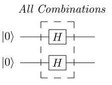
Generating All Combinations
To generate all possible quantum states of
![]() qubits, apply an H gate
on each qubit. For two qubits, the circuit shown in the
following figure generated all four quantum states:
qubits, apply an H gate
on each qubit. For two qubits, the circuit shown in the
following figure generated all four quantum states:
The top and bottom H gates each split
the ![]() qubit as follows:
qubit as follows:
Thus, the mega-qubit after each qubit is acted on by the respective H gate is:
This mega-qubit has four qubelet combinations, as shown in the following figure:
Each qubelet combination corresponds to one of the four
possible states of two qubits: ![]() ,
,
![]() ,
, ![]() ,
or
,
or ![]() .
.
Tagging the Best
After applying the H gates to the qubits, the mega-qubit holds all possible solutions to the application problem, including the optimal qubelet combination. The challenge in designing a quantum algorithm, then, is to remove the non-optimal quantum states. Grover’s algorithm is a way to retain a specific qubelet combination in the mega-qubit while removing the others. To illustrate how Grover’s algorithm goes about eliminating non-optimal quantum states, we’ll initially assume that we know which qubelet combination in the mega-qubit is optimal. Of course, in a real application, you’d like your program to find the optimal solution. So in Tagging When You Don’t Know the Optimal Solution, you’ll learn to design a quantum circuit that doesn’t require you to identify up front the optimal quantum state.
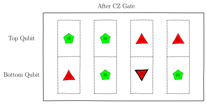
For now, though, suppose we want to retain the fourth
qubelet combination, ![]() .
We can achieve this by
applying a Controlled Z (CZ) gate,
described in Controlled Z (CZ) Gate,
as shown in the following circuit:
.
We can achieve this by
applying a Controlled Z (CZ) gate,
described in Controlled Z (CZ) Gate,
as shown in the following circuit:
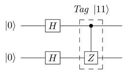
The CZ gate only affects the
![]() qubelet combination:
qubelet combination:
The other states’ qubelet combinations are left alone. The mega-qubit after applying the CZ gate is as shown in the following figure:

The inverted qubelet on the fourth qubelet combination,
corresponding to ![]() , is, thus,
tagged to differentiate it from the
others.
, is, thus,
tagged to differentiate it from the
others.
Qubelet Inversions Are Tied to the Equation for a Quantum State | |
|---|---|
|
|
Recall from Rotating Qubelets Through Any Angle,
the quantum state
The terms
So when one of them, say, the pentagon 
Noting that |
The quantum state, ![]() ,
of this mega-qubit is:
,
of this mega-qubit is:
Or, in vector form:

The amplitude of the ![]() qubelet combination is negative; the others are
positive.
qubelet combination is negative; the others are
positive.
You can also confirm this on the IBM Quantum Computer by looking at the Statevector—a graphical view of the quantum state vector in which the amplitudes are shown as bars whose heights are their magnitudes and whose colors correspond to the complex component (relative orientation between the qubelets)—as shown in the following figure:
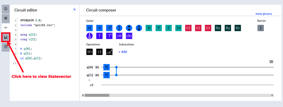
You’ll see a graphical view of the quantum vector, as shown in the following figure:

The four idealized states are shown as bars whose
heights are the amplitudes. The color of the bar
indicates the sign of the amplitude. The lighter
colored bar on the extreme right, corresponding to
![]() , indicates its amplitude
is negative.
, indicates its amplitude
is negative.
You can reason similarly to tag another state, for instance,
![]() , where
q[0]=1 and q[1]=0.
When we tagged
, where
q[0]=1 and q[1]=0.
When we tagged ![]() , we
applied a CZ gate so that the
bottom triangle
, we
applied a CZ gate so that the
bottom triangle ![]() qubelet
could be inverted. Thus, to tag
qubelet
could be inverted. Thus, to tag ![]() ,
where the second qubit, q[1], is
,
where the second qubit, q[1], is
![]() , you need to first switch it
to
, you need to first switch it
to ![]() . To this end, consider
the following circuit:
. To this end, consider
the following circuit:
Even though you can analyze this circuit with
matrices and confirm that the amplitude of the
![]() qubelet combination
is negative, you should be able to reason this
out in your mind as follows:
qubelet combination
is negative, you should be able to reason this
out in your mind as follows:
-
To tag
 where the bottom qubit is
  ,
the bottom qubit must first be switched to
,
the bottom qubit must first be switched to
 before being fed to the
target of the CZ
gate.
before being fed to the
target of the CZ
gate.
The mega-qubit after the first set of H gates on the left and the first X gate on the bottom qubit, before the target of the CZ gate, is as shown in the following figure:

-
The CZ gate only affects the
 qubelet combination,
the third column in the previous figure,
and inverts the bottom triangle
qubelet as shown in the figure.
qubelet combination,
the third column in the previous figure,
and inverts the bottom triangle
qubelet as shown in the figure.
Thus, the qubelet combination
will have a negative sign.
-
Finally, to switch
 to
to
 , apply an X
gate to the bottom qubit again. The X gate
toggles the bottom qubelets in all qubelet combinations,
as shown in the following figure:
, apply an X
gate to the bottom qubit again. The X gate
toggles the bottom qubelets in all qubelet combinations,
as shown in the following figure:
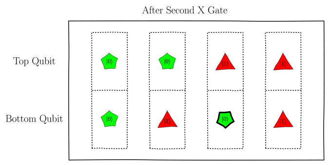
The bottom qubelet in the third column is switched to a pentagon
qubelet
and the others are restored to their original
qubelet types before the first X gate
was applied to both qubits.
As a result of these operations, the mega-qubit
![]() is:
is:
Or, in vector form:

The amplitude of the ![]() qubelet combination is negative and the others are
positive. The
qubelet combination is negative and the others are
positive. The ![]() qubelet
combination is, thus, tagged.
qubelet
combination is, thus, tagged.
You can check the Statevector on the IBM Quantum Computer’s console. This time, it’ll be as shown in the following figure.
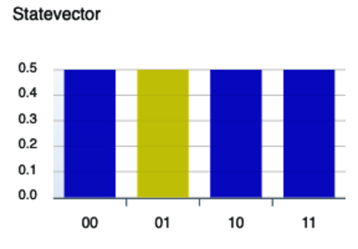
The lighter colored bar, indicating a negative
amplitude, is associated with 01.
But, in the discussion above, we wrote the
state as ![]() , which
is the reverse of the way that the
IBM Quantum Computer console writes it. Thus,
01 on the console actually corresponds to the
tagged state
, which
is the reverse of the way that the
IBM Quantum Computer console writes it. Thus,
01 on the console actually corresponds to the
tagged state ![]() .
.
Using Drag-and-Drop to Build the Circuit Gives You Insight | |
|---|---|
|
|
Dragging and dropping gates from the palette while keeping the Statevector tab active lets you see how the circuit modifies the quantum states as you add gates. You’ll notice that some gates barely affect the states, but other placements introduce large scale changes in the quantum state. |
In summary, then, to tag a particular qubelet combination, its amplitude has a different sign, achieved by inverting one of its qubelets, than the other combinations or idealized states. If you measured the qubits at this stage, however, then despite the amplitude of the tagged qubelet combination being negative, the mega-qubit formed by the two qubits would collapse to all four quantum states with roughly equal probability. That is, there seems to be no preference yet to tagging the optimal qubelet combinations. In the next section, you’ll see how the untagged qubelet combinations are removed from the mega-qubit.
The Tagging Circuit for ![]() illustrates a trademark feature of quantum
computing: gates that reverse the action of those
applied earlier, such as the
X gate after the CZ
gate. In conventional programming, after writing
a statement that, for example, increments a variable, it
would be unusual to decrement it later if
there was no computational logic dictating it.
Yet this quirky way of programming is a hallmark
of quantum computing.
illustrates a trademark feature of quantum
computing: gates that reverse the action of those
applied earlier, such as the
X gate after the CZ
gate. In conventional programming, after writing
a statement that, for example, increments a variable, it
would be unusual to decrement it later if
there was no computational logic dictating it.
Yet this quirky way of programming is a hallmark
of quantum computing.
The reason for this seemingly redundant way of hooking up gates in quantum computers is because you’re working with many states at the same time. When you applied the first X gate on the bottom qubit, it switched the bottom qubelets for all the qubelet combinations, not just the one that had to be tagged. So after you’re done dealing with the tagged qubelet combination by applying the CZ gate, you need to reverse the action of the first X gate and restore the other qubelet combinations back to their original states. This way, you can focus the quantum effects on specific qubelet combinations even though the quantum computer deals with all of them at the same time.
Canceling Circuit
To identify the tagged qubelet combinations representing the optimal solutions for your application, you need to remove the others from the mega-qubit. We’ll call this part of the program that eliminates the non-tagged qubelet combinations the Canceling Circuit.
The design of the Canceling Circuit illustrates why designing quantum circuits is vexing and puts a spotlight on a crucial aspect: when analyzing quantum circuits, even though your attention is on one set of states, always bear in mind that this set is just one of the many qubelet combinations in the mega-qubit associated with the circuit. What gates you apply to one state are simultaneously applied to the other combinations. It’s imperative that you keep the other states on your radar. Consequently, designing an algorithm is a combination of pattern extrapolation—a quantum effect for two qubits is extended to more qubits—applying matrices to portions of a circuit to precisely work out how gates modify quantum states and a healthy dose of guesswork or trial-and-error to calibrate the quantum effects. You’ll get lost in minutiae if you try to be absolutely precise. Rather, you’ll see how by using intuition and heuristic arguments, you can turn general ideas of quantum effects into workable code. By the end of this chapter, you’ll have a pattern that you can use to solve larger applications with more qubits.
In the Canceling Circuit, in particular, you have to eliminate several non-tagged states. What you do to remove one state impacts the others too. So you can’t just focus on one non-tagged state at a time. You have to think broadly first before zeroing in on specific gates.
Begin, then, by identifying at a high level the quantum effects you’ll need to use, as we’ll describe next.
Tagging Quantum States
With so many non-tagged and tagged states, it seems reasonable to expect that some form tagging will be used. Ironically, you’ll be tagging non-tagged states, as those are the ones that need to be eliminated.
Whatever states you end up deciding to tag, it’ll likely be when certain conditions are met. Thus, you’ll use a Controlled Z or CZ gate here, as shown in the following figure:

For most gates, you want to add a second one to reverse its effects (known as "backing out"). This time, you won’t do that because you want to retain the tagged solution—it’s the main purpose of this section of your program.
The matrix ![]() for this CZ
gate is:
for this CZ
gate is:

Splitting Qubits
No amount of rotating the qubelets in the non-tagged qubelet combinations will get rid of them: operations you apply on one will also be applied to the others, so there’s no net effect. Thus, paradoxically, to remove the non-tagged quantum states or qubelet combinations from the mega-qubit, you need to introduce additional qubelet combinations in the mix to provide opportunities for qubelet combinations to cancel.
Specifically, begin by applying an H gate to each qubit, as shown in the following figure:

The dots indicate that other gates will be added later to this circuit.
Following the procedure in
Two-Qubit Gate Matrices,
the matrix ![]() defining these
stacked H gates is:
defining these
stacked H gates is:
Before moving on to the next step in the design, back out these gates as you saw in Why the Second X Gate?, so that whichever qubelet combinations you don’t want to affect get restored back to their original states, as shown in the following figure:
The dots indicate that you’ll have other gates before the H gates are backed out.
Finding Asymmetry
Thus far, despite creating more qubelet combinations by splitting qubits, the overall mega-qubit is still somewhat symmetric in the sense that there are an equal number of each type of qubelet combination in the mega-qubit. To tilt the odds toward the optimal solution, you need to introduce asymmetry to favor some qubelet combinations over others. Moreover, whatever you do must work regardless of the quantum state that’s tagged. That is, just as we needed to introduce H gates to add more qubelet combinations to increase opportunities to cancel, we’ll need to first find symmetries.
Look again at the ![]() matrix
shown previously. Each column spells out how the gates
modify the idealized state corresponding to
that column. Specifically, each element
in the column will tell you how the gate
affects each of the idealized states when they
act on the qubelet combination corresponding to
that column. For example, the third column
stipulates that the
matrix
shown previously. Each column spells out how the gates
modify the idealized state corresponding to
that column. Specifically, each element
in the column will tell you how the gate
affects each of the idealized states when they
act on the qubelet combination corresponding to
that column. For example, the third column
stipulates that the ![]() qubelet combination in the mega-qubit is
modified as follows:
qubelet combination in the mega-qubit is
modified as follows:

Likewise, the second column tells you how the
![]() qubelet combination
is affected:
qubelet combination
is affected:

Compare the two quantum states: you’ll see that,
for instance, the ![]() qubelet combination has a positive sign
from the gates acting on
qubelet combination has a positive sign
from the gates acting on ![]() and a negative sign when they act on
and a negative sign when they act on
![]() .
.
In fact, by evaluating how all other idealized states
are modified by the circuit, you’ll notice that
![]() is the only qubelet combination
that always retains the same sign for any idealized state.
(You can also see that the first row of
is the only qubelet combination
that always retains the same sign for any idealized state.
(You can also see that the first row of ![]() is the only one in which every element has the same sign.)
is the only one in which every element has the same sign.)
This, then, is the lever we’re looking for.
![]() is the only qubelet
combination that will consistently appear in the
mega-qubit after the H gates,
regardless of which quantum state is tagged by
the Tagging Circuit.
is the only qubelet
combination that will consistently appear in the
mega-qubit after the H gates,
regardless of which quantum state is tagged by
the Tagging Circuit.
Tagging ![]()
To tag ![]() , using the
same logic outlined for tagging
, using the
same logic outlined for tagging ![]() in Tagging the Best, place
X gates as shown in the following
figure:
in Tagging the Best, place
X gates as shown in the following
figure:

These X gates need to be backed out since they’re only used as an intermediate step so that the non-tagged qubelet combinations are consistently tagged.
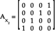
The matrix ![]() for these stacked
X gates is:
for these stacked
X gates is:
The CZ gate tags the ![]() qubelet combination so that it’s not restored by the
“backing-out” gates as the other combinations
are. But, and this is a very important point, keeping
these combinations in the mega-qubit regardless of which
state is tagged forces some other qubelet
combinations to cancel out so that the overall probability
of the mega-qubit collapsing to some state continues to
be 1.
qubelet combination so that it’s not restored by the
“backing-out” gates as the other combinations
are. But, and this is a very important point, keeping
these combinations in the mega-qubit regardless of which
state is tagged forces some other qubelet
combinations to cancel out so that the overall probability
of the mega-qubit collapsing to some state continues to
be 1.
At this point you have a design that breaks the symmetry in the mega-qubit. So it’s worthwhile now to precisely see how these non-optimal qubelet combinations are canceled out. To this end, break up the circuit into parts, as shown in the following circuit:

The label above each part is the matrix describing
the operation of that part. For example,
![]() is the matrix that shows how a
two-qubit quantum state is changed when each qubit is
acted on by an H gate.
is the matrix that shows how a
two-qubit quantum state is changed when each qubit is
acted on by an H gate.
The matrix ![]() for the
Canceling Circuit is
the following product of these matrices:
for the
Canceling Circuit is
the following product of these matrices:
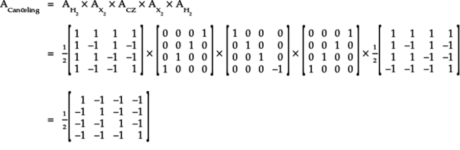
Remember that the order of multiplying matrices is opposite to that in which the corresponding parts of the circuit they describe appear.
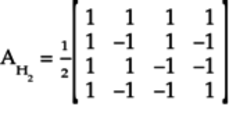
This matrix has both positive and negative terms in each column. In particular, the positive terms appear on the diagonal of the matrix and the negatives on the non-diagonal terms. These negative terms will be instrumental in wiping out the non-optimal states.
To see how the Canceling Circuit
removes the non-tagged qubelet combinations,
multiply its matrix ![]() with the vector
with the vector ![]() for the
for the ![]() tagged state:
tagged state:

In other words,
Even though the last remaining state,
![]() , after
all the others have been eliminated, has a negative sign,
when it collapses, 10
will still be recorded in the classical register.
, after
all the others have been eliminated, has a negative sign,
when it collapses, 10
will still be recorded in the classical register.
Multiplying matrices to get the matrix for the
Canceling Circuit,
![]() , looks formidable.
But, since
, looks formidable.
But, since ![]() and
and ![]() are their own inverses, the multiplication for
are their own inverses, the multiplication for
![]() can be rewritten as:
can be rewritten as:
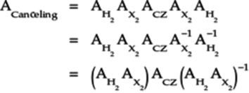
The last equation is obtained by noting that
![]() .
.
In this form, the matrix equation is the conjugate found in group theory:[65]
Here, ![]() and
and ![]() are generic
matrices, or transformations, that describe how
the state of a system changes by these two
transformations, respectively. The conjugate is
an “almost-inverse” in that it restores
most of the qubelets back to their original states,
except the ones that have to be retained.
are generic
matrices, or transformations, that describe how
the state of a system changes by these two
transformations, respectively. The conjugate is
an “almost-inverse” in that it restores
most of the qubelets back to their original states,
except the ones that have to be retained.
Don’t confuse this conjugate with complex conjugates discussed earlier. The group theory conjugates have a rich connection with quantum mechanics. (See Group Theory and its Application to the Quantum Mechanics of Atomic Spectra [WG59] for more information. The author was awarded the Nobel Prize in Physics in 1963[66] for introducing group theory in quantum mechanics. Another classic is The Theory of Groups and Quantum Mechanics [WR14]. Warning: these books are highly theoretical and not needed for quantum computing. I’ve mentioned them here to emphasize the deep connection between the matrix method for analyzing circuits and the group theoretic formulation of quantum mechanics.)
Notice the way the terms in the previous
equation cancel out: the negative terms pair up
with the positive terms in each element of the
quantum state vector, except for the element that
will remain.
That is, the non-tagged qubelet combinations, ![]() ,
,
![]() , and
, and ![]() ,
are removed from the mega-qubit.
,
are removed from the mega-qubit.
We didn’t explicitly work out the
Canceling Circuit by analyzing
how the pentagon ![]() and
triangle
and
triangle ![]() qubelets
form qubelet combinations that are transformed
by the circuit. Doing so would have been painfully
tedious and error-prone—and not particularly
enlightening. With the stack of H
gates at the beginning and end of
the Canceling Circuit acting on
blended states to begin with, you end up
with too many split qubelets to keep organized.
Rather, thinking holistically but still in terms of
rotating and toggling qubelets, and how these operations
in turn affect qubelet combinations, will guide you better
as you design your own algorithms.
qubelets
form qubelet combinations that are transformed
by the circuit. Doing so would have been painfully
tedious and error-prone—and not particularly
enlightening. With the stack of H
gates at the beginning and end of
the Canceling Circuit acting on
blended states to begin with, you end up
with too many split qubelets to keep organized.
Rather, thinking holistically but still in terms of
rotating and toggling qubelets, and how these operations
in turn affect qubelet combinations, will guide you better
as you design your own algorithms.
It may, though, seem that we somehow got lucky with the way we designed the Canceling Circuit to get the non-tagged states to cancel out. In fact, when dealing with larger numbers of qubits, the chances of getting all the non-tagged to cancel out are unlikely. But, as you’ll see in the next section, you can apply the concept multiple times to whittle away at the non-tagged states in each iteration by reducing the probabilities of the qubits collapsing to these non-tagged qubelet combinations at each iteration.
Canceling by Any Other Name Is ... Amplification | |
|---|---|
|
|
In the literature, the Canceling Circuit is described as reflection about the “average value of all the amplitudes” followed by “amplification” of the tagged state. See, for example, Grover himself explaining it here.[67] This characterization makes for some nice graphics of bars turning upside down and contracting. But I find this way of thinking hard to connect back to what’s happening in the quantum machine and, more importantly, extracting design principles from it to develop algorithms for other types of applications. |
Multiple Iterations
In the case in the previous section, the negative terms in each column of the matrix neatly lined up so that the non-optimal qubelet combinations got eliminated. When your application has to deal with many qubits, the math may not always work out so neatly. In fact, you’ll have to iterate the Tagging and Canceling circuits a few times to remove the non-optimal qubelet combinations.
In general, the number of iterations depends on the
number, ![]() , of qubits in your circuit:
, of qubits in your circuit:
The symbol ![]() is the Big-O
function that indicates the complexity of the
algorithm (loosely speaking, the number of iterations)
in terms of the number of variables. We expect that
the number of iterations will increase as your problem
size increases. But you want to strive to design
algorithms where the growth in iterations isn’t
exponential, making them impossible to implement
on actual machines.
is the Big-O
function that indicates the complexity of the
algorithm (loosely speaking, the number of iterations)
in terms of the number of variables. We expect that
the number of iterations will increase as your problem
size increases. But you want to strive to design
algorithms where the growth in iterations isn’t
exponential, making them impossible to implement
on actual machines.
Thus, the overall structure of Grover’s algorithm is as shown in the figure.

Putting the Quantum Effects Together
Going back to the two-qubit circuits that implement the quantum effects, connect them up in sequence, as shown in the following diagram:
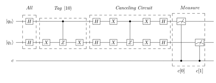
The quantum program describing this circuit is shown below:
| | // Initialize Quantum and Classical Registers |
| | qreg q[2]; |
| | creg c[2]; |
| | |
| | // Generate All Combinations |
| | h q[0]; |
| | h q[1]; |
| | |
| | // Tag |10> Quantum State |
| | x q[1]; |
| | cz q[0],q[1]; |
| | id q[0]; // Dummy gate for visually lining up circuit |
| | x q[1]; |
| | |
| | // Canceling Circuit |
| | h q[0]; |
| | h q[1]; |
| | x q[0]; |
| | x q[1]; |
| | cz q[0],q[1]; |
| | x q[0]; |
| | x q[1]; |
| | h q[0]; |
| | h q[1]; |
| | |
| | // Collapse Qubits |
| | measure q[0] -> c[0]; |
| | measure q[1] -> c[1]; |
Executing this circuit cancels out all the qubelet
combinations except for the tagged one,
![]() . The output of this
program is shown in the following figure:
. The output of this
program is shown in the following figure:
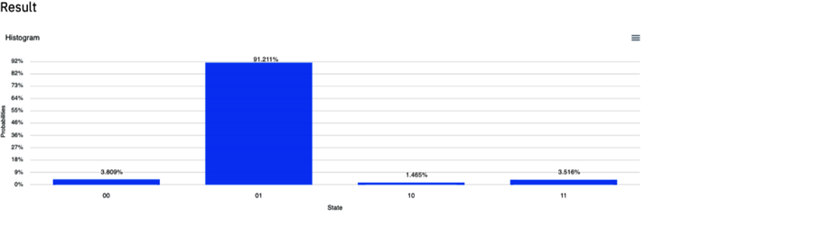
This output was obtained by running on a real
quantum computer. The 01 state has
highest probability of being observed in the
classical register. Because the IBM Quantum Computer
labels the bars opposite of our convention, the
01 state actually corresponds to 10.
This indicates that the two qubits collapsed to
![]() , the
tagged state. (The other states are the result of
noise when running on a real quantum computer.)
, the
tagged state. (The other states are the result of
noise when running on a real quantum computer.)
Optimizing Your Quantum Programs | |
|---|---|
|
|
As you hook up the tagging and canceling blocks, you’ll frequently see back-to-back H or back-to-back X gates. Since these gates restore the qubit to the state before these gates were applied, you can remove them when they occur in your code. |
Now that you’ve seen how these quantum effects come together to eliminate non-tagged quantum states, in the next section, you’ll begin to put these effects together to hunt for optimal solutions for realistic applications.