Working with Matrices and Vectors

In quantum mechanics, we frequently multiply matrices as well as matrices with vectors. As shown in "Fundamental Theorem of Linear Algebra" [Str93], although the mechanics of these types of multiplications may seem arbitrary, they offer a point of view that gives us a way to represent the operation of gates on quantum states. (For a lucid description of linear algebra in a practical setting, especially the discussion relating to the columns of a matrix, which is of the most interest to us, see Foundations of Network Optimization and Games [FB16].)

A matrix is an array of numbers arranged as follows:

In this matrix, the numbers are organized in two rows and two columns. Although in quantum computing we’ll deal with square matrices in which the number of rows are the same as that for columns, here we’ll work with rectangular matrices, where the number of rows differs from that for columns, to emphasize that there’s nothing special about square matrices in this regard.

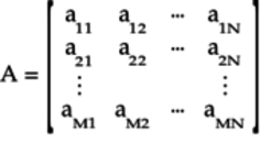
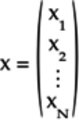
It’ll be more instructive to talk about matrices whose elements are represented symbolically, as shown here:

(The “” is just a shortcut to indicate that the matrix contains other elements or numbers that are labeled in the same way.) The elements, or numbers, , where and , of the matrix are laid out in an array of rows and columns. The first subscript is the index of the row, and the second subscript is the index of the column in the array. Thus, the element refers to the number in the first row and second column of the matrix. The number of rows and columns of the array are the dimensions of the matrix, which we’ll write as .

A vector is a matrix with just one column:

This vector has rows or elements and is an vector.

Multiplying the matrix with the vector , we get:

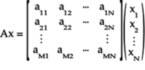
The product will be an vector of elements, as shown here:

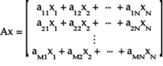
Each element in this vector is obtained by multiplying term-by-term the -th row with the elements of the vector . Thus, for the second element in this vector, we multiplied each term in the second row with the corresponding elements in the vector. (Because each term in a row of the matrix is multiplied by the corresponding element in the vector , the number of columns in the matrix has to equal the number of elements of the vector .)

Key Step

The critical step is to group the terms associated with each , as a sum of vectors, as follows:

Each column of the matrix is multiplied by the corresponding element of the vector . In other words, vectors can be interpreted as a way of extracting just the column we want from a matrix.

To see how vectors act like column selectors, consider the following vector whose second element is a 1, and the others are 0:

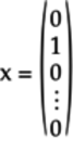
Substituting this vector in the previous equation, we get:

That is, only the second column is multiplied by 1, the other columns are multiplied by 0. In other words, we have effectively pulled out the second column of the matrix .

Multiplying Matrices

The idea of using vectors as selectors can be applied to multiplying matrices as well:

• Treat the second matrix as a collection of columns or vectors.
• Then, obtain each column of the product by multiplying the first matrix by the corresponding column of the second matrix.

For example, suppose you’re multiplying the following matrices:

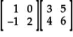
Think of the second matrix as a collection of the following columns or vectors:

The first column of the product is:

The second column of the product is:

To get the product of the matrices, put the two columns together:

If you’re not in the business of multiplying matrices, the method described here may be at odds with the traditional way in which each element of the product matrix is calculated by doing an element-by-element multiplication of each row of the first matrix by each column of the second matrix and then summing each individual multiplication. The method described in this section moves the focus from individual elements and puts the emphasis on columns, a view that mathematicians prefer, as it gives a physical interpretation instead of merely a bunch of calculations. You’ll find this meaning of the vector for the qubits as a column selector more fitting when modeling quantum gates and analyzing quantum circuits.

Using a Computer Algebra System for Multiplying Matrices and Vectors

When analyzing and building algorithms for quantum computers, you’ll multiply matrices and vectors. To avoid tediously multiplying these by hand, especially as the number of matrices and their sizes gets large, you can use an online mathematical system such as Sage Mathematical Software System^[108] or SageMath. SageMath has a web-based interface called SageMathCell^[109] which lets you perform quick calculations by directly entering your equations on a web page.

In computer algebra systems, matrices are defined as an array of arrays. That is, the matrix is an array whose elements are arrays themselves. Each array element corresponds to a row of the matrix. For example, consider the matrix here:

To enter this matrix in SageMathCell, define an array in which each element is another array, one for each of the three rows as follows:

The function matrix() then converts the array of arrays to a matrix for the computer algebra system.

Likewise, consider the following vector:

You would enter this vector in SageMathCell as follows:

The function vector() converts this array into a vector for the computer algebra system.

To multiply the matrix with the vector , you enter . (Note that you must use the operator to indicate multiplication.) SageMathCell then returns the vector .

Several other functions, such as inverting matrices, are available. Check out the quick-reference wiki for a list of the commonly used functions.^[110]