Two-Qubit Gate Matrices

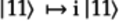
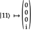
Just as the columns of a single-qubit gate matrix correspond to the idealized states, the columns of a matrix representing a two-qubit gate, such as the ​Controlled NOT (CNOT) Gate​, correspond to the four idealized states—, , , and — for two qubits:

The letters are complex numbers with the usual conjugates .

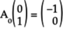
Each column is the action of the gate on the idealized state associated with that column. For example, look at the ​Controlled NOT (CNOT) Gate​ gate in which the control qubit is set to and its target to , as shown in the following figure:

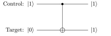
Because the control is , the target qubit is switched to .

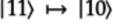
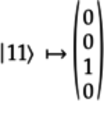
Or, the state is changed by the CNOT gate to the state. To express this operation as a matrix column, write the latter as a vector:

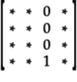
Thus, the third column of the matrix for the CNOT gate is:

Similarly, you can fill the other columns:

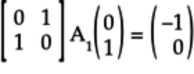
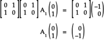
CNOT acts on

When the control qubit is , the target qubit continues to be . Thus, or:

CNOT acts on

Since the control qubit is , the target qubit is unaffected and continues to . Thus, or:

CNOT acts on

In this case, the control qubit is . So, the target qubit switches from to . Thus, or:

Putting these vectors as the appropriate columns in the previous matrix, we’ll get the CNOT gate’s matrix :

Notice that we’ve suppressed the column labels, but you should still associate each column with the corresponding idealized states.

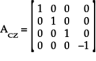
Following the same line of reasoning, you can derive the gate matrix for the ​Controlled Z (CZ) Gate​. The CZ gate only rotates the triangle qubelet on the target qubit when the control bit is , as shown in the following figure:

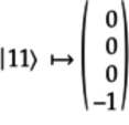
That is, the state becomes . Writing the latter as a vector:

The CZ gate leaves the other idealized states alone. Or, in terms of vectors:

In the first two instances, the control qubit is . Thus, the target qubit is unchanged. In the last case, even though the control qubit is , the target qubit is and not affected by the CZ gate.

These vectors form the rest of the columns of the CZ gate’s matrix :

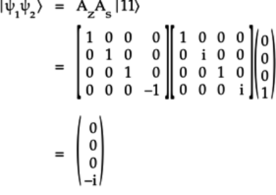
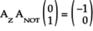
With matrices for two-qubit gates, you can follow the procedure in ​Sequence of Gates as Matrix Multiplication​, to work out how circuits with two-qubit gates modify quantum states. For example, see the following circuit:

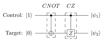
Obtain the two-qubit quantum state as follows:

Notice the order of the multiplication of the and matrices is reverse that of the order in which the corresponding gates are applied to the input state in the quantum circuit. Also, in the previous equation, the input state is replaced with a vector which has a 1 in the third element, corresponding to .

The result of this multiplication is a vector whose last element is . The bottom element is associated with the quantum state . So, a value indicates that this sequence of gates changes the quantum state as follows:

For this circuit, you can verify this result by manually working out the action of the gates on the qubits: the control qubit is 1, the CNOT gate switches the bottom qubit to , which the CZ gate then inverts to . This corresponds to the quantum state , as found earlier using matrices and vectors. As the number of gates increases, this sort of analysis becomes tedious and error-prone. But the matrix approach always works.

Matrix and Vector Multiplication Isn’t a Replacement for Quantum Computing

You may get the idea that multiplying gate matrices with the vector for a quantum state is really all that it takes to do quantum computations. In fact, this principle drives many simulators in various computer languages. But as the number of qubits increases, classical computers would grind to a halt as they run out of resources trying to do matrix math. Quantum computers, on the other hand, are impervious to this excessive workload, as they work with the mega-qubit using quantum mechanical principles instead of using classical means. Still, the matrix method is important to learn since it gives you a way to analyze small portions of a circuit and see how the qubelets are affected. If you try to use Measure gates instead, you won’t get a complete picture of how the rotations of the qubelets of different qubits interact.

You can apply this technique of multiplying quantum state vectors with gate matrices as long as your quantum circuit only has two-qubit gates. In the next section, you’ll learn to include single-qubit gates that switch, split, and rotate qubelets on one or both qubits in your quantum circuits.

Circuits with Single- and Two-Qubit Gates

When designing your own quantum programs you’ll frequently want to apply a single-qubit gate on one or both qubits in addition to the two-qubit gates. For example, consider the following circuit:

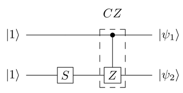
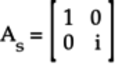
A single-qubit S gate is applied on the bottom qubit before it’s fed to the target of the CZ gate. So, this circuit contains the single-qubit S gate coupled with the two-qubit CZ gate. In other words, you end up with a situation where you have to deal with the matrix for the S gate as well as the matrix for the CZ gate.

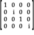
To apply the matrix method to calculate the quantum states of the qubits in this circuit, the matrices need to be compatible so that they can be multiplied. For square matrices, this means that the matrices must have the same dimensions.

Thus, the single-qubit S gate is “made” into a two-qubit gate by appending the second qubit, the top one in this case, as a pass-through, as shown in the following figure:^[44][45]

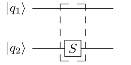
Next, use the single-qubit S gate’s matrix as a guide to calculate the matrix for the two-qubit S gate. For reference, the matrix for the ​S Gate​, is:

Notice that this matrix implies that the pentagon qubelets are unaffected, while the triangle qubelets are rotated by radians, or 90° anticlockwise:

The angle indicates the relative difference between the pentagon and triangle qubelets.

As we did for the CNOT gate earlier in this section, work out the columns of the matrix by seeing what this circuit does to each of the four idealized states, , , , and :

Idealized State:

The top qubit, , is a pass-through. So it’s unchanged by the gate.

The bottom qubit, , is fed to the S gate. From this gate’s matrix, , the bottom qubit, is also unaffected.

Thus, . Write the latter state as a vector:

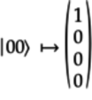
Note that the first element of this vector is associated with .

Idealized State:

The top qubit, , is a pass-through. So, it’s unchanged by the gate.

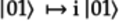The bottom qubit, , becomes when acted on by the S gate in accordance with the gate matrix . Thus, . Write the latter state as a vector:

The second element, associated with , is .

Idealized State:

The top qubit, , is a pass-through. So it’s unchanged by the gate.

The bottom qubit, , is fed to the S gate and is unchanged in accordance with the gate matrix . Thus, 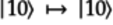. Write the latter state as a vector:

The third element is associated with .

Idealized State:

The top qubit, , is a pass-through. So it’s unchanged by the gate.

The bottom qubit, , becomes when acted on by the S gate in accordance with the gate matrix . Thus, . Write the latter state as a vector:

These vectors then form the columns of the matrix for the pass-through two-qubit S gate:

Now, the matrices for both the pass-through S gate and the CZ gate are the same size. Thus, you can multiply their matrices to get how these gates act on :

Notice that the order of multiplying the matrices and is opposite to the order in which the corresponding gates are applied to the input state . Also, the input state is replaced with its vector in the previous equation.

Quantum Circuit Synthesis, or Guess the Gate

The gate matrix technique is a useful tool to analyze how gates modify quantum states. But they can also guide you to select gates that transform a given quantum state to another. For example, suppose you want to take a state that has a triangle qubelet to one that has an inverted pentagon qubelet, as shown in the following figure:

The vector for the quantum state with the single triangle qubelet is:

And, the vector for the quantum state after the quantum operations is:

Thus, you can represent this change of state by the following equation:

The matrix represents a sequence of quantum operations implemented by hooking up quantum gates. To determine the gate matrices that underpin these quantum operations, apply matrix operations to tease apart to reveal the gates.

Since a triangle qubelet on the left is switched to a pentagon qubelet on the right, albeit inverted, it seems reasonable that a NOT gate will be a part of this sequence of gates. So, modify the matrix by “pulling” the matrix for the NOT gate out, as follows:

Substituting for in the previous equation:

As still needs to be determined, simplify the left hand side by multiplying both sides by the Hermitian transpose of :

Thus, represents a gate that leaves the pentagon qubelets alone but inverts the triangle qubelets. That is, represents a Z gate.

In other words, the triangle qubelet can be made into an inverted pentagon qubelet by first applying the NOT gate, followed by the Z gate. This operation is expressed as follows:

Notice that the gate matrices are written in the order opposite in which they’re applied to the qubit.

We’re making the assumption that the NOT gate is applied last. If it turns out that we hit a dead end and are unable to get the quantum state we want, we try other placements of the NOT gate’s matrix .

The multiplication of the matrices with the vector for results in the quantum state :

Once again, to convince yourself that the matrix procedure gives the correct result, you can reason this circuit out manually: the S gate on the bottom qubit, , rotates its triangle qubelet by radians, or a quarter turn anticlockwise. Since, the control qubit to the CZ gate is , the CZ gate will rotate the triangle qubelet on the target qubit on the bottom by a half turn. So, the triangle qubelet will end up rotated a quarter turn clockwise, or radians, as shown in the figure.

Analyzing existing circuit designs is useful to pick up ways to work with qubits. But eventually you’ll want to twist qubelets in ways unique to your application. So in the next section, you’ll learn how matrices also help to identify the gates you’ll need in your own designs.

The circuits in this section were initialized with idealized states. In the next section, you’ll learn to work with circuits seeded with blended states obtained as a result of a previous computation.