Idealized States Redux—Multi-Qubit Version
Before learning to precisely manipulate multiple qubits in quantum circuits, like you did with single qubits in Chapter 6, Designer Genes—Custom Quantum States, and Chapter 7, Small Step for Man—Single Qubit Programs, you need to augment your understanding of idealized states.
Idealized States for One Qubit
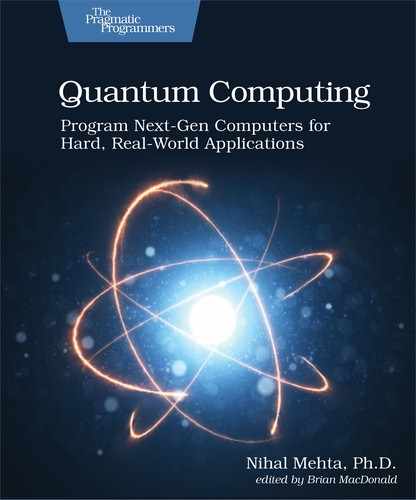
The idealized states for single qubits are the two
ways that it can collapse. Consider, for example,
a qubit having five pentagon ![]() and two triangle
and two triangle ![]() qubelets (both
rotated), as shown in the following figure:
qubelets (both
rotated), as shown in the following figure:
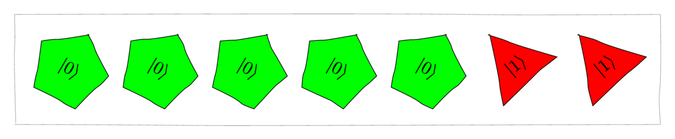
Regardless of how the pentagon ![]() and triangle
and triangle ![]() qubelets are rotated,
this qubit collapses in one of the following two ways:
qubelets are rotated,
this qubit collapses in one of the following two ways:
- Collapses to

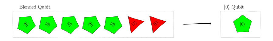
- Collapses to

Of course, the qubit would collapse more frequently to
![]() than
than ![]() because the qubit has a greater number of pentagon
because the qubit has a greater number of pentagon
![]() qubelets than triangle
qubelets than triangle
![]() qubelets. But it would always
collapse to one of these two types.
qubelets. But it would always
collapse to one of these two types.
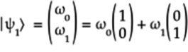
Thus, as in Quantum States and Probabilities,
any quantum state ![]() can be expressed in terms of the idealized states
can be expressed in terms of the idealized states
![]() and
and ![]() ,
as follows:
,
as follows:
The parameters ![]() and
and ![]() are the amplitudes associated with the idealized states.
By setting different values for the amplitudes
are the amplitudes associated with the idealized states.
By setting different values for the amplitudes
![]() and
and ![]() ,
you can specify any quantum state.
And the subscript on the quantum state
,
you can specify any quantum state.
And the subscript on the quantum state ![]() indicates that it’s a quantum state for a single qubit.
indicates that it’s a quantum state for a single qubit.
In terms of vectors, as shown in Quantum States as Vectors,
the quantum state ![]() can also
be written as:
can also
be written as:
Idealized States for Two Qubits
When dealing with two qubits, the situation is similar:
each qubit collapses to either ![]() or
or ![]() . Thus, we can write the
ways that two qubits collapse as follows:
. Thus, we can write the
ways that two qubits collapse as follows:
|
Qubit 1 |
Qubit 2 |
|---|---|
|
|
|
|
|
|
|
|
|
|
|
|
Thus, the idealized states of the two qubits are as follows:
These, then, are the 22, or 4,
idealized states for two qubits, and any
two-qubit quantum state can be expressed in terms of these
four idealized states. Specifically, if the quantum state of
the first qubit is ![]() and that of the second is
and that of the second is ![]() ,
then the quantum state of the two-qubit system
is written as
,
then the quantum state of the two-qubit system
is written as ![]() .
.
The coefficients ![]() ,
, ![]() ,
,
![]() , and
, and ![]() are
the amplitudes of the idealized states
are
the amplitudes of the idealized states
![]() ,
, ![]() ,
,
![]() , and
, and ![]() ,
respectively.
,
respectively.
Since the two qubits can only collapse to these four idealized states, the probabilities of collapsing to them, the “squares” of the amplitudes—an amplitude multiplied by its conjugate—sum up to 1:
The quantum state of a two-qubit system is completely defined by these four amplitudes. It’s also expressed by the vector shown.
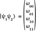
This vector, in turn, can be written in terms of the four idealized states:

Since there are four idealized states, the quantum
state of a two-qubit system will be a ![]() vector. Specifically, the vectors for the four idealized
states are:
vector. Specifically, the vectors for the four idealized
states are:

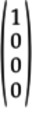
Each element in the vector corresponds to an
idealized state. So, the first element is associated
with ![]() , the second with
, the second with
![]() , and so on, till the last
with
, and so on, till the last
with ![]() .
.
These idealized states aren’t just theoretical concepts. They underpin all quantum programs, as shown in the next section.
Idealized States and Quantum Programs
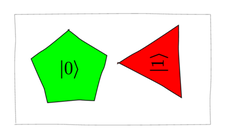
Idealized states are closely intertwined with quantum programs—they’re the outputs. Consider, for example, the two-qubit quantum circuit shown in the following figure:

Analyze this circuit by first looking at each qubit individually:
- Qubit q[0]
-
No gates act on the q[0] qubit:

- Qubit q[1]
-
The H gate splits the
qubit in q[0] to a pentagon
qubelet and a triangle qubelet.
The S gate then rotates the triangle
qubelet 90°, or a
quarter turn clockwise, as shown in the following
figure:
Alternatively, you can also use the gate matrices (see Classifying Quantum Gates) and the vector for the idealized state
, as follows:
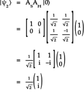
This vector indicates that the quantum state
 is made up
of a pentagon qubelet
and a triangle qubelet
rotated 90° anticlockwise.
is made up
of a pentagon qubelet
and a triangle qubelet
rotated 90° anticlockwise.
But, because this is a quantum circuit, there’s an
additional step that has no classical
equivalent: the formation of the mega-qubit, as
described in
Multi-Qubit Superposition: The Mega-Qubit,
to get the quantum state ![]() of the two-qubit circuit.
of the two-qubit circuit.
The pentagon ![]() qubelet in the
top qubit q[0] pairs up with the qubelets
in the bottom qubit q[1] to give the mega-qubit
shown in the figure.
qubelet in the
top qubit q[0] pairs up with the qubelets
in the bottom qubit q[1] to give the mega-qubit
shown in the figure.

This mega-qubit can collapse to either of the two qubelet combinations with equal probability. To get the quantum state of the mega-qubit, normalize the chances of picking a qubelet combination by following the procedure similar to that described in Normalizing Qubelets, but apply it for qubelet combinations instead of qubelets:
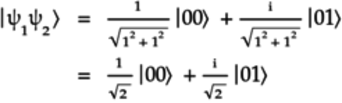
The triangle ![]() qubelet
at the bottom of the second qubelet combination
is rotated a quarter turn anticlockwise.
As a result you see the complex number
qubelet
at the bottom of the second qubelet combination
is rotated a quarter turn anticlockwise.
As a result you see the complex number ![]() associated with the second term.
associated with the second term.
Since this qubit has two qubelet combinations, it collapses in one of the following two ways:
- Collapses to

-
When this mega-qubit is measured, the qubelet combination on the left is selected roughly 50% of the time and collapses to
, as shown here:

This corresponds to the following vector:
- Collapses to

-
When this mega-qubit is measured, the qubelet combination on the right is selected roughly 50% of the time and collapses to
, as shown in the
following figure:
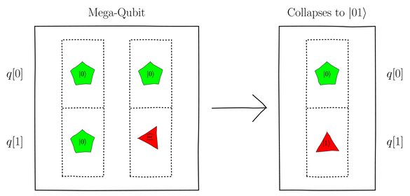
Although rotated qubelets play a pivotal role in quantum effects such as entangling and canceling qubelets, when a qubit collapses, qubelets are reset to their non-rotated orientations. Thus, the rotated triangle
qubelet snaps back
to the non-rotated position.
The collapsed qubelet combination corresponds to the following vector:

You can verify that this circuit does indeed work as the analysis just described by running it on the IBM Quantum Computer. The code listing for this circuit is as follows:
| 1: | qreg q[2]; |
| 2: | creg c[2]; |
| 3: | |
| 4: | h q[1]; |
| 5: | s q[1]; |
| 6: | measure q[0] -> c[0]; |
| 7: | measure q[1] -> c[1]; |
The H and S gates acting on the q[1] qubit are declared on lines 4 and 5, respectively, followed by the Measure gates.
The output of this program running on a real quantum computer is shown in the following figure:
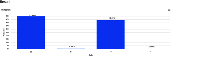
This program collapses to the two binary states
00 and 10 roughly half the time.
The other two states are just noise when using
a real quantum computer. Because of the
way that IBM’s classical register is structured
(see Using the IBM Computer: Multi-Bit Classical Register),
the highest numbered classical bit, in this case
c[1], is written first. Thus, the
10 state corresponds to c[1]c[0],
which, in turn, records the qubits q[1]q[0].
Hence, the measured classical states 00
and 01 correspond to ![]() and
and ![]() , respectively. In other words, the measured classical states
reflect the idealized states.
, respectively. In other words, the measured classical states
reflect the idealized states.
Idealized States for Three or More Qubits
Determining the idealized states for three or more qubits
is analogous: document the ways that the qubits
collapse. For example, a three-qubit quantum state
![]() collapses
to the following
collapses
to the following ![]() vectors:
vectors:

The idealized states for ![]() qubits follow
a similar pattern: you’ll end up with 2n
states. As
qubits follow
a similar pattern: you’ll end up with 2n
states. As ![]() —the number of qubits in
your program—grows, the number of idealized states
grows exponentially and become impossible to write down.
But the mega-qubit is able to handle all these states
simultaneously. So, whereas it’s difficult
for a classical computer to work with them, a quantum
computer merely needs
—the number of qubits in
your program—grows, the number of idealized states
grows exponentially and become impossible to write down.
But the mega-qubit is able to handle all these states
simultaneously. So, whereas it’s difficult
for a classical computer to work with them, a quantum
computer merely needs ![]() qubits, a far smaller
number, to work with.
qubits, a far smaller
number, to work with.
In the next section, you’ll see how the idealized states are intimately tied to the gate matrix.