
5
Interprocess Communication Based on Shared Variables
CONTENTS
5.1 Race Conditions and Critical Regions
5.2 Hardware-Assisted Lock Variables
5.3 Software-BasedMutual Exclusion
More often than not, in both general-purpose and real-time systems, processes do not live by themselves and are not independent of each other. Rather, several processes are brought together to form the application software, and they must therefore cooperate to solve the problem at hand.
Processes must therefore be able to communicate, that is, exchange information, in a meaningful way. As discussed in Chapter 2, it is quite possible to share some memory among processes in a controlled way by making part of their address space refer to the same physical memory region.
However, this is only part of the story. In order to implement a correct and meaningful data exchange, processes must also synchronize their actions in some ways. For instance, they must not try to use a certain data item if it has not been set up properly yet. Another purpose of synchronization, presented in Chapter 4, is to regulate process access to shared resources.
This chapter addresses the topic, explaining how shared variables can be used for communication and introducing various kinds of hardware- and software-based synchronization approaches.
5.1 Race Conditions and Critical Regions
At first sight, using a set of shared variables for interprocess communication may seem a rather straightforward extension of what is usually done in sequential programming. In a sequential program written in a high-level language, it is quite common to have a set of functions, or procedures, that together form the application and exchange data exactly in the same way: there is a set of global variables defined in the program, all functions have access to them (within the limits set forth by the scoping rules of the programming language), and they can get and set their value as required by the specific algorithm they implement.
A similar thing also happens at the function call level, in which the caller prepares the function arguments and stores them in a well-known area of memory, often allocated on the stack. The called function then reads its arguments from there and uses them as needed. The value returned by the function is handled in a similar way. When possible, for instance, when the function arguments and return value are small enough, the whole process may be optimized by the language compiler to use some processor registers instead of memory, but the general idea is still the same.
Unfortunately, when trying to apply this idea to a concurrent system, one immediately runs into several, deep problems, even in trivial cases. If we want, for instance, to count how many events of a certain kind happened in a sequential programming framework, it is quite intuitive to define a memory-resident, global variable (the definition will be somewhat like int k if we use the C programming language) and then a very simple function void inck(void) that only contains the statement k = k+1.
It should be pointed out that, as depicted in Figure 5.1, no real-world CPU is actually able to increment k in a single, indivisible step, at least when the code is compiled into ordinary assembly instructions. Indeed, even a strongly simplified computer based on the von Neumann architecture [31, 86] will perform a sequence of three distinct steps:
Load the value of
kfrom memory into an internal processor register; on a simple processor, this register would be the accumulator. From the processor’s point of view, this is an external operation because it involves both the processor itself and memory, two distinct units that communicate through the memory bus. The load operation is not destructive, that is,kretains its current value after it has been performed.Increment the value loaded from memory by one. Unlike the previous one, this operation is internal to the processor. It cannot be observed from the outside, also because it does not require any memory bus cycle to be performed. On a simple processor, the result is stored back into the accumulator.
Store the new value of
kinto memory with an external operation involving a memory bus transaction like the first one. It is important to notice that the new value ofkcan be observed from outside the processor only at this point, not before. In other words, if we look at memory,kretains its original value until this final step has been completed.
Even if real-world architectures are actually much more sophisticated than what is shown in Figure 5.1—and a much more intimate knowledge of their intricacies is necessary to precisely analyze their behavior—the basic reasoning is still the same: most operations that are believed to be indivisible at the programming language level (even simple, short statements like k = k+1), eventually correspond to a sequence of steps when examined at the instruction execution level.
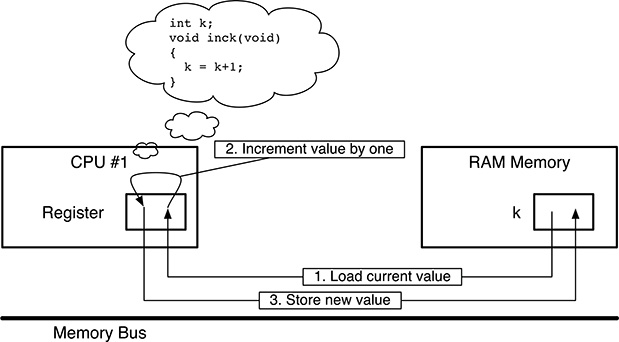
FIGURE 5.1
Simplified representation of how the CPU increments a memory-resident variable k.
However, this conceptual detail is often overlooked by many programmers because it has no practical consequences as long as the code being considered is executed in a strictly sequential fashion. It becomes, instead, of paramount importance as soon as we add concurrency to the recipe.
Let us imagine, for example, a situation in which not one but two different processes want to concurrently update the variable k because they are both counting events belonging to the same class but coming from different sources. Both of them use the same code, that is, function inck(), to perform the update.
For simplicity, we will assume that each of those two processes resides on its own physical CPU, and the two CPUs share a single-port memory by means of a common memory bus, as is shown in Figure 5.2. However, the same argument still holds, even if the processes share the same physical processor, by using the multiprogramming techniques discussed in Chapter 3.
Under those conditions, if we let the initial value of k be 0, the following sequence of events may occur:
1.1. CPU #1 loads the value of k from memory and stores it into one of its registers, R1. Since k currently contains 0, R1 will also contain 0.
1.2. CPU #1 increments its register R1. The new value of R1 is therefore 1.
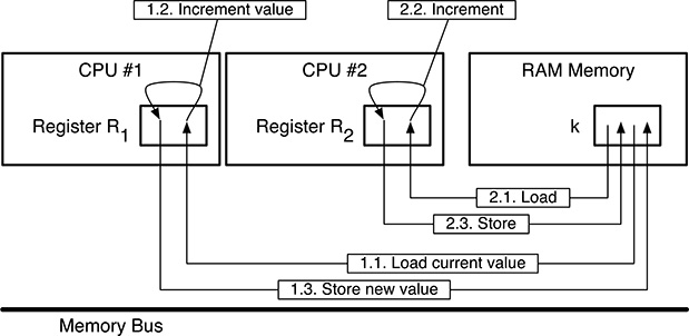
FIGURE 5.2
Concurrently incrementing a shared variable in a careless way leads to a race condition.
2.1. Now CPU #2 takes over, loads the value of k from memory, and stores it into one of its registers, R2. Since CPU #1 has not stored the updated value of R1 back to memory yet, CPU #2 still gets the value 0 from k, and R2 will also contain 0.
2.2. CPU #2 increments its register R2. The new value of R2 is therefore 1.
2.3. CPU #2 stores the contents of R2 back to memory in order to update k, that is, it stores 1 into k.
1.3. CPU #1 does the same: it stores the contents of R1 back to memory, that is, it stores 1 into k.
Looking closely at the sequence of events just described, it is easy to notice that taking an (obviously correct) piece of sequential code and using it for concurrent programming in a careless way did not work as expected. That is, two distinct kinds of problems arose:
In the particular example just made, the final value of
kis clearly incorrect: the initial value ofkwas 0, two distinct processes incremented it by one, but its final value is 1 instead of 2, as it should have been.The second problem is perhaps even worse: the result of the concurrent update is not only incorrect but it is incorrect only sometimes. For example, the sequence 1.1, 1.2, 1.3, 2.1, 2.2, 2.3 leads to a correct result.
In other words, the value and correctness of the result depend on how the elemental steps of the update performed by one processor interleave with the steps performed by the other. In turn, this depends on the precise timing relationship between the processors, down to the instruction execution level. This is not only hard to determine but will likely change from one execution to another, or if the same code is executed on a different machine.
Informally speaking, this kind of time-dependent errors may be hard to find and fix. Typically, they take place with very low probability and may therefore be very difficult to reproduce and analyze. Moreover, they may occur when a certain piece of machinery is working in the field and no longer occur during bench testing because the small, but unavoidable, differences between actual operation and testing slightly disturbed system timings.
Even the addition of software-based instrumentation or debugging code to a concurrent application may subtly change process interleaving and make a time-dependent error disappear. This is also the reason why software development techniques based on concepts like “write a piece of code and check whether it works or not; tweak it until it works,” which are anyway questionable even for sequential programming, easily turn into a nightmare when concurrent programming is involved.
These observations also lead to the general definition of a pathological condition, known as race condition, that may affect a concurrent system: whenever a set of processes reads and/or writes some shared data to carry out a computation, and the results of this computation depend on the exact way the processes interleaved, there is a race condition.
In this statement, the term “shared data” must be construed in a broad sense: in the simplest case, it refers to a shared variable residing in memory, as in the previous examples, but the definition actually applies to any other kind of shared object, such as files and devices. Since race conditions undermine the correctness of any concurrent system, one of the main goals of concurrent programming will be to eliminate them altogether.
Fortunately, the following consideration is of great help to better focus this effort and concentrate only on a (hopefully small) part of the processes’ code. The original concept is due to Hoare [36] and Brinch Hansen [15]:
A process spends part of its execution doing internal operations, that is, executing pieces of code that do not require or make access to any shared data. By definition, all these operations cannot lead to any race condition, and the corresponding pieces of code can be safely disregarded when the code is analyzed from the concurrent programming point of view.
Sometimes a process executes a region of code that makes access to shared data. Those regions of code must be looked at more carefully because they can indeed lead to a race condition. For this reason, they are called critical regions or critical sections.
With this definition in mind, and going back to the race condition depicted in Figure 5.2, we notice that both processes have a critical region, and it is the body of function inck(). In fact, that fragment of code increments the shared variable k. Even if the critical region code is correct when executed by one single process, the race condition stems from the fact that we allowed two distinct processes to be in their critical region simultaneously.
We may therefore imagine solving the problem by allowing only one process to be in a critical region at any given time, that is, forcing the mutual exclusion between critical regions pertaining to the same set of shared data. For the sake of simplicity, in this book, mutual exclusion will be discussed in rather informal and intuitive terms. See, for example, the works of Lamport [57, 58] for a more formal and general treatment of this topic.
In simple cases, mutual exclusion can be ensured by resorting to special machine instructions that many contemporary processor architectures support. For example, on the Intel® 64 and IA-32 architecture [45], the INC instruction increments a memory-resident integer variable by one.
When executed, the instruction loads the operand from memory, increments it internally to the CPU, and finally stores back the result; it is therefore subject to exactly the same race condition depicted in Figure 5.2. However, it can be accompanied by the LOCK prefix so that the whole sequence is executed atomically, even in a multiprocessor or multicore environment.
Unfortunately, these ad-hoc solutions, which coerce a single instruction to be executed atomically, cannot readily be applied to more general cases, as it will be shown in the following example. Figure 5.3 shows a classic way of solving the so-called producers–consumers problem. In this problem, a group of processes P1, ..., Pn, called producers, generate data items and make them available to the consumers by means of the prod() function. On the other hand, another group of processes C1, ..., Cm, the consumers, use the cons() function to get hold of data items.
To keep the code as simple as possible, data items are assumed to be integer values, held in int-typed variables. For the same reason, the error-handling code (which should detect and handle any attempt of putting a data item into a full buffer or, symmetrically, getting an item from an empty buffer) is not shown.
With this approach, producers and consumers exchange data items through a circular buffer with N elements, implemented as a shared, statically allocated array int buf[N]. A couple of shared indices, int in and int out, keep track of the first free element of the buffer and the oldest full element, respectively. Both of them start at zero and are incremented modulus N to circularize the buffer. In particular,
Assuming that the buffer is not completely full, the function
prod()first storesd, the data item provided by the calling producer, intobuf[in], and then incrementsin. In this way,innow points to the next free element of the buffer.Assuming that the buffer is not completely empty, the function
cons()takes the oldest data item residing in the buffer frombuf[out], stores it into the local variablec, and then incrementsoutso that the next consumer will get a fresh data item. Last, it returns the value ofcto the calling consumer.
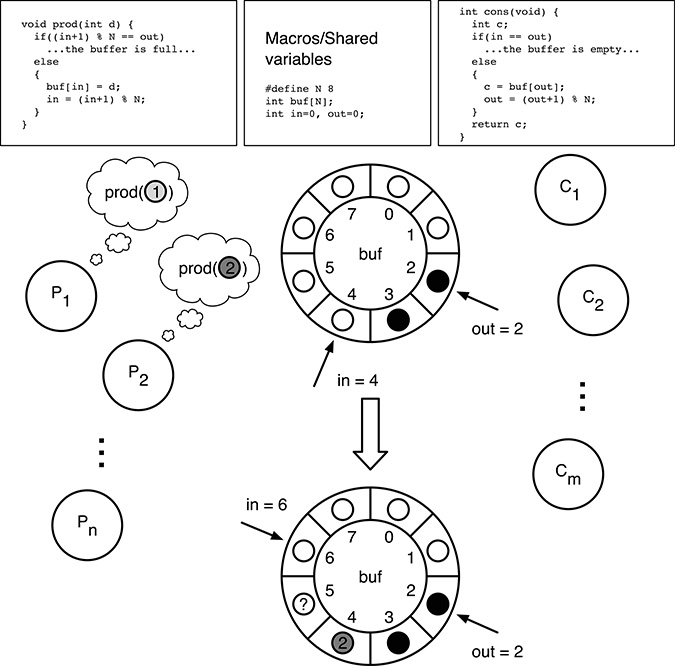
FIGURE 5.3
Not all race conditions can be avoided by forcing a single instruction to be executed atomically.
If should be noted that, since the condition in == out would be true not only for a buffer that is completely empty but also for a buffer containing N full elements, the buffer is never filled completely in order to avoid this ambiguity. In other words, we must consider the buffer to be full even if one free element—often called the guard element—is still available. The corresponding predicate is therefore (in+1) % N == out. As a side effect of this choice, of the N buffer elements, only up to N − 1 can be filled with data.
Taking for granted the following two, quite realistic, hypotheses:
any integer variable can be loaded from, or stored to, memory with a single, atomic operation;
neither the processor nor the memory access subsystem reorders memory accesses;
it is easy to show that the code shown in Figure 5.3 works correctly for up to one producer and one consumer running concurrently.
For processors that reorder memory accesses—as most modern, high-performance processors do—the intended sequence can be enforced by using dedicated machine instructions, often called fences or barriers. For example, the SFENCE, LFENCE, and MFENCE instructions of the Intel® 64 and IA-32 architecture [45] provide different degrees of memory ordering.
The SFENCE instruction is a store barrier; it guarantees that all store operations that come before it in the instruction stream have been committed to memory and are visible to all other processors in the system before any of the following store operations becomes visible as well. The LFENCE instruction does the same for memory load operations, and MFENCE does it for both memory load and store operations.
On the contrary, and quite surprisingly, the code no longer works as it should as soon as we add a second producer to the set of processes being considered. One obvious issue is with the increment of in (modulus N), but this is the same issue already considered in Figure 5.2 and, as discussed before, it can be addresses with some hardware assistance. However, there is another, subtler issue besides this one.
Let us consider two producers, P1 and P2: they both concurrently invoke the function prod() to store an element into the shared buffer. For this example, let us assume, as shown in Figure 5.3, that P1 and P2 want to put the values 1 and 2 into the buffer, respectively, although the issue does not depend on these values at all.
It is also assumed that the shared buffer has a total of 8 elements and initially contains two data items, represented as black dots, whereas white dots represent empty elements. Moreover, we assume that the initial values of in and out are 4 and 2, respectively. This is the situation shown in the middle of the figure. The following interleaving could take place:
Process P1 begins executing
prod(1)first. Sinceinis 4, it stores 1 intobuf[4].Before P1 makes further progress, P2 starts executing
prod(2).The value ofinis still 4, hence P2 stores 2 intobuf[4]and overwrites the data item just written there by P1.At this point, both P1 and P2 increment
in. Assuming that the race condition issue affecting these operations has been addressed, the final value ofinwill be 6, as it should.
It can easily be seen that the final state of the shared variables after these operations, shown in the lower part of Figure 5.3, is severely corrupted because:
the data item produced by P1 is nowhere to be found in the shared buffer: it should have been in
buf[4], but it has been overwritten by P2;the data item
buf[5]is marked as full becauseinis 6, but it contains an undefined value (denoted as “?” in the figure) since no data items have actually been written into it.
From the consumer’s point of view, this means that, on the one hand, the data item produced by P1 has been lost and the consumer will never get it. On the other hand, the consumer will get and try to use a data item with an undefined value, with dramatic consequences.
With the same reasoning, it is also possible to conclude that a very similar issue also occurs if there is more than one consumer in the system. In this case, multiple consumers could get the same data item, whereas other data items are never retrieved from the buffer. From this example, two important conclusions can be drawn:
The correctness of a concurrent program does not merely depend on the presence or absence of concurrency, as it happens in very simple cases, such as that shown in Figure 5.2, but it may also depend on how many processes there are, the so-called degree of concurrency. In the last example, the program works as long as there are only two concurrent processes in the system, namely, one producer and one consumer. It no longer works as soon as additional producers (or consumers) are introduced.
Not all race conditions can be avoided by forcing a single instruction to be executed atomically. Instead, we need a way to force mutual exclusion at the critical region level, and critical regions may comprise a sequence of many instructions. Going back to the example of Figure 5.3 and considering how critical regions have been defined, it is possible to conclude that the producers’ critical region consists of the whole body of
prod(), while the consumers’ critical region is the whole body ofcons(), except for thereturnstatement, which only operates on local variables.
The traditional way of ensuring the mutual exclusion among critical region entails the adoption of a lock-based synchronization protocol. A process that wants to access a shared object, by means of a certain critical region, must perform the following sequence of steps:
Acquire some sort of lock associated with the shared object and wait if it is not immediately available.
Use the shared object.
Release the lock, so that other processes can acquire it and be able to access the same object in the future.
In the above sequence, step 2 is performed by the code within the critical region, whereas steps 1 and 3 are a duty of two fragments of code known as the critical region entry and exit code. In this approach, these fragments of code must compulsorily surround the critical region itself. If they are relatively short, they can be incorporated directly by copying them immediately before and after the critical region code, respectively.
If they are longer, it may be more convenient to execute them indirectly by means of appropriate function calls in order to reduce the code size, with the same effect. In the examples presented in this book, we will always follow the latter approach. This also highlights the fact that the concept of critical region is related to code execution, and not to the mere presence of some code between the critical region entry and exit code. Hence, for example, if a function call is performed between the critical region entry and exit code, the body of the called function must be considered as part of the critical region itself.
In any case, four conditions must be satisfied in order to have an acceptable solution [85]:
It must really work, that is, it must prevent any two processes from simultaneously executing code within critical regions pertaining to the same shared object.
Any process that is busy doing internal operations, that is, is not currently executing within a critical region, must not prevent other processes from entering their critical regions, if they so decide.
If a process wants to enter a critical region, it must not have to wait forever to do so. This condition guarantees that the process will eventually make progress in its execution.
It must work regardless of any low-level details about the hardware or software architecture. For example, the correctness of the solution must not depend on the number of processes in the system, the number of physical processors, or their relative speed.
In the following sections, a set of different lock-based methods will be discussed and confronted with the correctness conditions just presented. It should, however, be noted that lock-based synchronization is by far the most common, but it is not the only way to solve the race condition problem. In Chapter 10, the disadvantages of the lock-based approach will be highlighted, and several other methods that function without using any kind of lock will be briefly presented.
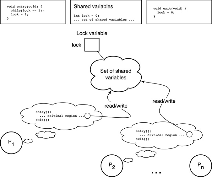
FIGURE 5.4
Lock variables do not necessarily work unless they are handled correctly.
5.2 Hardware-Assisted Lock Variables
A very simple way of ensuring the mutual exclusion among multiple processes wanting to access a set of shared variables is to uniquely associate a lock variable with them, as shown in Figure 5.4. If there are multiple, independent sets of shared variables, there will be one lock variable for each set.
The underlying idea is to use the lock variable as a flag that will assume two distinct values, depending on how many processes are within their critical regions. In our example, the lock variable is implemented as an integer variable (unsurprisingly) called lock, which can assume either the value 0 or 1:
0 means that no processes are currently accessing the set of shared variables associated with the lock;
1 means that one process is currently accessing the set of shared variables associated with the lock.
Since it is assumed that no processes are within a critical region when the system is initialized, the initial value of lock is 0. As explained in Section 5.1, each process must surround its critical regions with the critical region entry and exit code. In Figure 5.4, this is accomplished by calling the entry() and exit() functions, respectively.
Given how the lock variable has been defined, the contents of these functions are rather intuitive. That is, before entering a critical section, a process P must
Check whether the lock variable is 1. If this is the case, another process is currently accessing the set of shared variables protected by the lock. Therefore, P must wait and perform the check again later. This is done by the
whileloop shown in the figure.When P eventually finds that the lock variable is 0, it breaks the
whileloop and is allowed to enter its critical region. Before doing this, it must set the lock variable to 1 to prevent other processes from entering, too.
The exit code is even simpler: whenever P is abandoning a critical region, it must reset the lock variable to 0. This may have two possible effects:
If one or more processes are already waiting to enter, one of them will find the lock variable at 0, will set it to 1 again, and will be allowed to enter its critical region.
If no processes are waiting to enter, the lock variable will stay at 0 for the time being until the critical region entry code is executed again.
Unfortunately, this naive approach to the problem does not work even if we consider only two processes P1 and P2. This is due to the fact that, as described above, the critical region entry code is composed of a sequence of two steps that are not executed atomically. The following interleaving is therefore possible:
1.1. P1 executes the entry code and checks the value of lock, finds that lock is 0, and immediately escapes from the while loop.
2.1. Before P1 had the possibility of setting lock to 1, P2 executes the entry code, too. Since the value of lock is still 0, it exits from the while loop as well.
2.2. P2 sets lock to 1.
1.2. P1 sets lock to 1.
At this point, both P1 and P2 execute their critical code and violate the mutual exclusion constraint. An attentive reader would have certainly noticed that, using lock variables in this way, the mutual exclusion problem has merely been shifted from one “place” to another. Previously the problem was how to ensure mutual exclusion when accessing the set of shared variables, but now the problem is how to ensure mutual exclusion when accessing the lock variable itself.
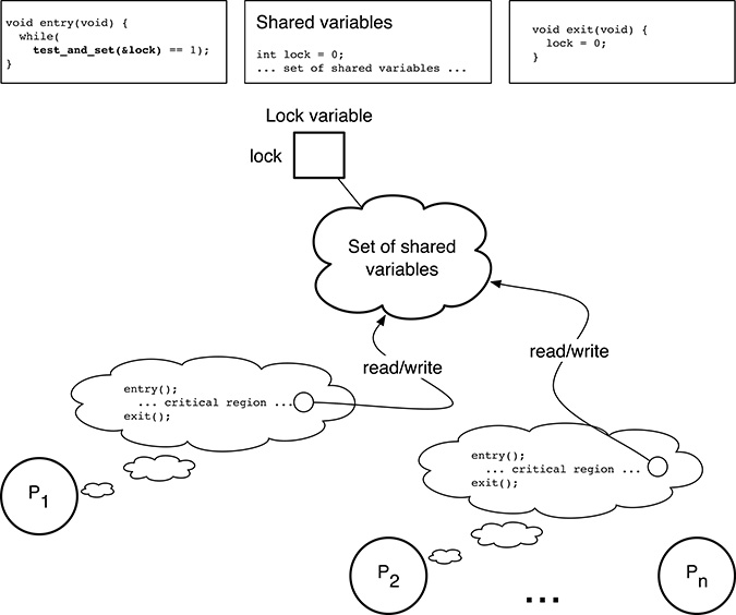
FIGURE 5.5
Hardware-assisted lock variables work correctly.
Given the clear similarities between the scenarios depicted in Figures 5.2 and 5.4, it is not surprising that the problem has not been solved at all. However, this is one of the cases in which hardware assistance is very effective. In the simplest case, we can assume that the processor provides a test and set instruction. This instruction has the address p of a memory word as argument and atomically performs the following three steps:
It reads the value
vof the memory word pointed byp.It stores 1 into the memory word pointed by
p.It puts
vinto a register.
As shown in Figure 5.5, this instruction can be used in the critical region entry code to avoid the race condition discussed before because it forces the test of lock to be atomic with respect to its update. The rest of the code stays the same. For convenience, the test and set instruction has been denoted as a C function int_test_and_set(int *p), assuming that the int type indeed represents a memory word.
For what concerns the practical implementation of this technique, on the Intel® 64 and IA-32 architecture [45], the BTS instruction tests and sets a single bit in either a register or a memory location. It also accepts the LOCK prefix so that the whole instruction is executed atomically.
Another, even simpler, instruction is XCHG, which exchanges the contents of a register with the contents of a memory word. In this case, the bus-locking protocol is activated automatically regardless of the presence of the LOCK prefix. The result is the same as the test and set instruction if the value of the register before executing the instruction is 1. Many other processor architectures provide similar instructions.
It can be shown that, considering the correctness conditions stated at the end of Section 5.1, the approach just described is correct with respect to conditions 1 and 2 but does not fully satisfy conditions 3 and 4:
By intuition, if one of the processes is noticeably slower that the others—because, for example, it is executed on a slower processor in a multiprocessor system—it is placed at a disadvantage when it executes the critical region entry code. In fact, it checks the
lockvariable less frequently than the others, and this lowers its probability of findinglockat 0. This partially violates condition 4.In extreme cases, the execution of the
whileloop may be so slow that other processes may succeed in taking turns entering and exiting their critical regions, so that the “slow” process never findslockat 0 and is never allowed to enter its own critical region. This is in contrast with condition 3.
From the practical standpoint, this may or may not be a real issue depending on the kind of hardware being used. For example, using this method for mutual exclusion among cores in a multicore system, assuming that all cores execute at the same speed (or with negligible speed differences), is quite safe.
5.3 Software-Based Mutual Exclusion
The first correct solution to the mutual exclusion problem between two processes, which does not use any form of hardware assistance, was designed by Dekker [23]. A more compact and elegant solution was then proposed by Peterson [71].
Even if Peterson’s algorithm can be generalized to work with an arbitrary (but fixed) number of processes, for simplicity we will only consider the simplest scenario, involving only two processes P0 and P1 as shown in Figure 5.6. It is also assumed that the memory access atomicity and ordering constraints set forth in Section 5.1 are either satisfied or can be enforced.
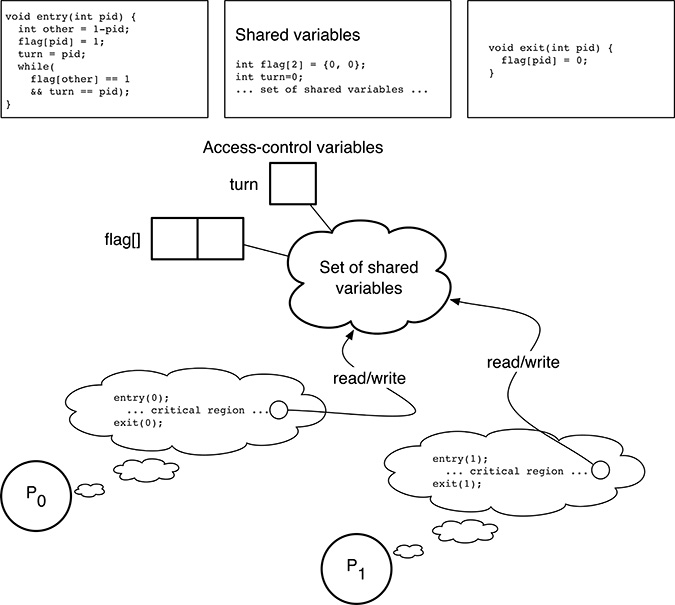
FIGURE 5.6
Peterson’s software-based mutual exclusion for two processes.
Unlike the other methods discussed so far, the critical region entry and exit functions take a parameter pid that uniquely identifies the invoking process and will be either 0 (for P0) or 1 (for P1). The set of shared, access-control variables becomes slightly more complicated, too. In particular,
There is now one flag for each process, implemented as an array
flag[2]of two flags. Each flag will be 1 if the corresponding process wants to, or succeeded in entering its critical section, and 0 otherwise. Since it is assumed that processes neither want to enter, nor already are within their critical region at the beginning of their execution, the initial value of both flags is 0.The variable
turnis used to enforce the two processes to take turns if both want to enter their critical region concurrently. Its value is a process identifier and can therefore be either 0 or 1. It is initially set to 0 to make sure it has a legitimate value even if, as we will see, this initial value is irrelevant to the algorithm.
A formal proof of the correctness of the algorithm is beyond the scope of this book, but it is anyway useful to gain an informal understanding of how it works and why it behaves correctly. As a side note, the same technique is also useful in gaining a better understanding of how other concurrent programming algorithms are designed and built.
The simplest and easiest-to-understand case for the algorithm happens when the two processes do not execute the critical region entry code concurrently but sequentially. Without loss of generality, let us assume that P0 executes this code first. It will perform the following operations:
It sets its own flag,
flag[0], to 1. It should be noted that P0 works onflag[0]becausepidis 0 in the instance ofenter()it invokes.It sets
turnto its own process identifierpid, that is, 0.It evaluates the predicate of the
whileloop. In this case, the right-hand part of the predicate is true (becauseturnhas just been set topid), but the left-hand part is false because the other process is not currently trying to enter its critical section.
As a consequence, P0 immediately abandons the while loop and is granted access to its critical section. The final state of the shared variables after the execution of enter(0) is
flag[0] == 1(it has just been set by P0);flag[1] == 0(P1 is not trying to enter its critical region);turn == 0(P0 has been the last process to start executingenter()).
If, at this point, P1 tries to enter its critical region by executing enter(1), the following sequence of events takes place:
It sets its own flag,
flag[1], to 1.It sets
turnto its own process identifier, 1.It evaluates the predicate of the
whileloop. Both parts of the predicate are true because:The assignment
other = 1-pidimplies that the value ofotherrepresents the process identifier of the “other” process. Therefore,flag[other]refers toflag[0], the flag of P0, and this flag is currently set to 1.The right-hand part of the predicate,
turn == pid, is also true becauseturnhas just been set this way by P1, and P0 does not modify it in any way.
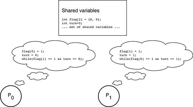
FIGURE 5.7
Code being executed concurrently by the two processes involved in Peterson’s critical region enter code.
P1 is therefore trapped in the while loop and will stay there until P0 exits its critical region and invokes exit(0), setting flag[0] back to 0. In turn, this will make the left-hand part of the predicate being evaluated by P1 false, break its busy waiting loop, and allow P1 to execute its critical region. After that, P0 cannot enter its critical region again because it will be trapped in enter(0).
When thinking about the actions performed by P0 and P1 when they execute enter(), just discussed above, it should be remarked that, even if the first program statement in the body of enter(), that is, flag[pid] = 1, is the same for both of them, the two processes are actually performing very different actions when they execute it.
That is, they are operating on different flags because they have got different values for the variable pid, which belongs to the process state. This further highlights the crucial importance of distinguishing programs from processes when dealing with concurrent programming because, as it happens in this case, the same program fragment produces very different results depending on the executing process state.
It has just been shown that the mutual exclusion algorithm works satisfactorily when P0 and P1 execute enter() sequentially, but this, of course, does not cover all possible cases. Now, we must convince ourselves that, for every possible interleaving of the two, concurrent executions of enter(), the algorithm still works as intended. To facilitate the discussion, the code executed by the two processes has been listed again in Figure 5.7, replacing the local variables pid and other by their value. As already recalled, the value of these variables depends on the process being considered.
For what concerns the first two statements executed by P0 and P1, that is, flag[0] = 1 and flag[1] = 1, it is easy to see that the result does not depend on the execution order because they operate on two distinct variables. In any case, after both statements have been executed, both flags will be set to 1.
On the contrary, the second pair of statements, turn = 0 and turn = 1, respectively, work on the same variable turn. The result will therefore depend on the execution order but, thanks to the memory access atomicity taken for granted at the single-variable level, the final value of turn will be either 0 or 1, and not anything else, even if both processes are modifying it concurrently. More precisely, the final value of turn only depends on which process executed its assignment last, and represents the identifier of that process.
Let us now consider what happens when both processes evaluate the predicate of their while loop:
The left-hand part of the predicate has no effect on the overall outcome of the algorithm because both
flag[0]andflag[1]have been set to one.The right-hand part of the predicate will be true for one and only one process. It will be true for at least one process because
turnwill be either 0 or 1. In addition, it cannot be true for both processes becauseturncannot assume two different values at once and no processes can further modify it.
In summary, either P0 or P1 (but not both) will be trapped in the while loop, whereas the other process will be allowed to enter into its critical region. Due to our considerations about the value of turn, we can also conclude that the process that set turn last will be trapped, whereas the other will proceed. As before, the while loop executed by the trapped process will be broken when the other process resets its flag to 0 by invoking its critical region exit code.
Going back to the correctness conditions outlined in Section 5.1, this algorithm is clearly correct with respect to conditions 1 and 2. For what concerns conditions 3 and 4, it also works better than the hardware-assisted lock variables discussed in Section 5.2. In particular,
The slower process is no longer systematically put at a disadvantage. Assuming that P0 is slower than P1, it is still true that P1 may initially overcome P0 if both processes execute the critical region entry code concurrently. However, when P1 exits from its critical region and then tries to immediately reenter it, it can no longer overcome P0.
When P1 is about to evaluate its
whileloop predicate for the second time, the value ofturnwill in fact be 1 (because P1 set it last), and both flags will be set. Under these conditions, the predicate will be true, and P1 will be trapped in the loop. At the same time, as soon asturnhas been set to 1 by P1, P0 will be allowed to proceed regardless of its speed because itswhileloop predicate becomes false and stays this way.For the same reason, and due to the symmetry of the code, if both processes repeatedly contend against each other for access to their critical region, they will take turns at entering them, so that no process can systematically overcome the other. This property also implies that, if a process wants to enter its critical region, it will succeed within a finite amount of time, that is, at the most the time the other process spends in its critical region.
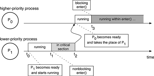
FIGURE 5.8
Busy wait and fixed-priority assignment may interfere with each other, leading to an unbounded priority inversion.
For the sake of completeness, it should be noted that the algorithm just described, albeit quite important from the historical point of view, is definitely not the only one of this kind. For instance, interested readers may want to look at the famous Lamport’s bakery algorithm [55]. One of the most interesting properties of this algorithm is that it still works even if memory read and writes are not performed in an atomic way by the underlying processor. In this way, it completely solves the mutual exclusion problem without any kind of hardware assistance.
5.4 From Active to Passive Wait
All the methods presented in Sections 5.2 and 5.3 are based on active or busy wait loops: a process that cannot immediately enter into its critical region is delayed by trapping it into a loop. Within the loop, it repeatedly evaluates a Boolean predicate that indicates whether it must keep waiting or can now proceed.
One unfortunate side effect of busy loops is quite obvious: whenever a process is engaged in one of those loops, it does not do anything useful from the application point of view—as a matter of fact, the intent of the loop is to prevent it from proceeding further at the moment—but it wastes processor cycles anyway. Since in many embedded systems processor power is at a premium, due to cost and power consumption factors, it would be a good idea to put these wasted cycles to better use.
Another side effect is subtler but not less dangerous, at least when dealing with real-time systems, and concerns an adverse interaction of busy wait with the concept of process priority and the way this concept is often put into practice by a real-time scheduler.
In the previous chapters it has already been highlighted that not all processes in a real-time system have the same “importance” (even if the concept of importance has not been formally defined yet) so that some of them must be somewhat preferred for execution with respect to the others. It is therefore intuitively sound to associate a fixed priority value to each process in the system according to its importance and design the scheduler so that it systematically prefers higher-priority processes when it is looking for a ready process to run.
The intuition is not at all far from reality because several popular real-time scheduling algorithms, to be discussed in Chapter 12, are designed exactly in this way. Moreover, Chapters 13–16 will also make clearer that assigning the right priority to all the processes, and strictly obeying them at run-time, also plays a central role to ensure that the system meets its timing requirements and constraints.
A very simple example of the kind of problems that may occur is given in Figure 5.8. The figure shows two processes, P0 and P1, being executed on a single physical processor under the control of a scheduler that systematically prefers P0 to P1 because P0’s priority is higher. It is also assumed that these two processes share some data and—being written by a proficient programmer who just read this chapter—therefore contain one critical region each. The critical regions are protected by means of one of the mutual exclusion methods discussed so far. As before, the critical region entry code is represented by the function enter(). The following sequence of events may take place:
Process P0 becomes ready for execution at t0, while P1 is blocked for some other reason. Supposing that P0 is the only ready process in the system at the moment, the scheduler makes it run.
At t1, P0 wants to access the shared data; hence, it invokes the critical region entry function
enter(). This function is nonblocking because P1 is currently outside its critical region and allows P0 to proceed immediately.According to the fixed-priority relationship between P0 and P1, as soon as P1 becomes ready, the scheduler grabs the processor from P0 and immediately brings P1 into the running state with an action often called preemption. In Figure 5.8, this happens at t2.
If, at t3, P1 tries to enter its critical section, it will get stuck in
enter()because P0 was preempted before it abandoned its own critical section.
It should be noted that the last event just discussed actually hides two distinct facts. One of them is normal, the other is not:
Process P1, the higher-priority process, cannot enter its critical section because it is currently blocked by P0, a lower-priority process. This condition is called priority inversion because a synchronization constraint due to an interaction between processes—through a set of shared data in this case—is going against the priority assignment scheme obeyed by the scheduler. In Figure 5.8, the priority inversion region is shown in dark gray.
Even if this situation may seem disturbing, it is not a problem by itself. Our lock-based synchronization scheme is indeed working as designed and, in general, a certain amount of priority inversion is unavoidable when one of those schemes is being used to synchronize processes with different priorities. Even in this very simple example, allowing P1 to proceed would necessarily lead to a race condition.
Unfortunately, as long as P1 is trapped in
enter(), it will actively use the processor—because it is performing a busy wait—and will stay in the running state so that our fixed-priority scheduler will never switch the processor back to P0. As a consequence, P0 will not further proceed with execution, it will never abandon its critical region, and P1 will stay trapped forever. More generally, we can say that the priority inversion region is unbounded in this case because we are unable to calculate a finite upper bound for the maximum time P1 will be blocked by P0.
It is also useful to remark that some priority relationships between concurrent system activities can also be “hidden” and difficult to ascertain because, for instance, they are enforced by hardware rather than software. In several operating system architectures, interrupt handling implicitly has a priority greater than any other kind of activity as long as interrupts are enabled. In those architectures, the unbounded priority situation shown in Figure 5.8 can also occur when P0 is a regular process, whereas P1 is an interrupt handler that, for some reason, must exchange data with P0. Moreover, it happens regardless of the software priority assigned to P0.
From Section 3.4 in Chapter 3, we know that the process state diagram already comprises a state, the Blocked state, reserved for processes that cannot proceed for some reason, for instance, because they are waiting for an I/O operation to complete. Any process belonging to this state does not proceed with execution but does so without wasting processor cycles and without preventing other processes from executing in its place. This kind of wait is often called passive wait just for this reason.
It is therefore natural to foresee a clever interaction between interprocess synchronization and the operating system scheduler so that the synchronization mechanism makes use of the Blocked state to prevent processes from running when appropriate. This certainly saves processor power and, at least in our simple example, also addresses the unbounded priority inversion issue. As shown in Figure 5.9, if enter() and exit() are somewhat modified to use passive wait,
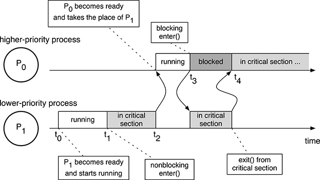
FIGURE 5.9
Using passive wait instead of busy wait solves the unbounded priority inversion problem in simple cases.
At t3, P1 goes into the Blocked state, thus performing a passive instead of a busy wait. The scheduler gives the processor to P0 because P1 is no longer ready for execution.
Process P0 resumes execution in its critical section and exits from it at t4 by calling
exit(). As soon as P0 exits from the critical section, P1 is brought back into the Ready state because it is ready for execution again.As soon as P1 is ready again, the scheduler reevaluates the situation and gives the processor back to P1 itself so that P1 is now running in its critical section.
It is easy to see that there still is a priority inversion region, shown in dark gray in Figure 5.9, but it is no longer unbounded. The maximum amount of time P1 can be blocked by P0 is in fact bounded by the maximum amount of time P0 can possibly spend executing in its critical section. For well-behaved processes, this time will certainly be finite.
Even if settling on passive wait is still not enough to completely solve the unbounded priority inversion problem in more complex cases, as will be shown in Chapter 15, the underlying idea is certainly a step in the right direction and led to a number of popular synchronization methods that will be discussed in the following sections.
The price to be paid is a loss of efficiency because any passive wait requires a few transition in the process state diagram, the execution of the scheduling algorithm, and a context switch. All these operations are certainly slower with respect to a tight, busy loop, which does not necessarily require any context switch when multiple physical processors are available. For this reason, busy wait is still preferred when the waiting time is expected to be small, as it happens for short critical regions, and efficiency is of paramount importance to the point that wasting several processor cycles in busy waiting is no longer significant.
This is the case, for example, when busy wait is used as a “building block” for other, more sophisticated methods based on passive wait, which must work with multiple, physical processors. Another field of application of busy wait is to ensure mutual exclusion between physical processors for performance-critical operating system objects, such as the data structures used by the scheduler itself.
Moreover, in the latter case, using passive wait would clearly be impossible anyway.
5.5 Semaphores
Semaphores were first proposed as a general interprocess synchronization framework by Dijkstra [23]. Even if the original formulation was based on busy wait, most contemporary implementations use passive wait instead. Even if semaphores are not powerful enough to solve, strictly speaking, any arbitrary concurrent programming problem, as pointed out for example in [53], they have successfully been used to address many problems of practical significance. They still are the most popular and widespread interprocess synchronization method, also because they are easy and efficient to implement.
A semaphore is an object that comprises two abstract items of information:
a nonnegative, integer value;
a queue of processes passively waiting on the semaphore.
Upon initialization, a semaphore acquires an initial value specified by the programmer, and its queue is initially empty. Neither the value nor the queue associated with a semaphore can be read or written directly after initialization. On the contrary, the only way to interact with a semaphore is through the following two primitives that are assumed to be executed atomically:
P(s), when invoked on semaphores, checks whether the value of the semaphore is (strictly) greater than zero.If this is the case, it decrements the value by one and returns to the caller without blocking.
Otherwise, it puts the calling process into the queue associated with the semaphore and blocks it by moving it into the Blocked state of the process state diagram.
V(s), when invoked on semaphores, checks whether the queue associated with that semaphore is empty or not.If the queue is empty, it increments the value of the semaphore by one.
Otherwise, it picks one of the blocked processes found in the queue and makes it ready for execution again by moving it into the Ready state of the process state diagram.
In both cases,
V(s)never blocks the caller. It should also be remarked that, whenV(s)unblocks a process, it does not necessarily make it running immediately. In fact, determining which processes must be run, among the Ready ones, is a duty of the scheduling algorithm, not of the interprocess communication mechanism. Moreover, this decision is often based on information—for instance, the relative priority of the Ready processes—that does not pertain to the semaphore and that the semaphore implementation may not even have at its disposal.
The process state diagram transitions triggered by the semaphore primitives are highlighted in Figure 5.10. As in the general process state diagram shown in Figure 3.4 in Chapter 3, the transition of a certain process A from the Running to the Blocked state caused by P() is voluntary because it depends on, and is caused by, a specific action performed by the process that is subjected to the transition, in this case A itself.
On the other hand, the transition of a process A from the Blocked back into the Ready state is involuntary because it depends on an action performed by another process. In this case, the transition is triggered by another process B that executes a V() involving the semaphore on which A is blocked. After all, by definition, as long as A is blocked, it does not proceed with execution and cannot perform any action by itself.
Semaphores provide a simple and convenient way of enforcing mutual exclusion among an arbitrary number of processes that want to have access to a certain set of shared variables. As shown in Figure 5.11, it is enough to associate a mutual exclusion semaphore mutex to each set of global variables to be protected. The initial value of this kind of semaphore is always 1.
Then, all critical regions pertaining to that set of global variables must be surrounded by the statements P(mutex) and V(mutex), using them as a pair of “brackets” around the code, so that they constitute the critical region entry and exit code, respectively.
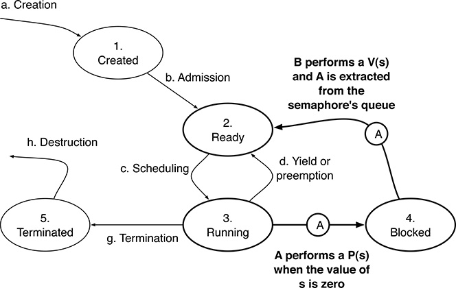
FIGURE 5.10
Process State Diagram transitions induced by the semaphore primitives P() and V().
In this chapter, we focus on the high-level aspects of using semaphores. For this reason, in Figure 5.11, we assume that a semaphore has the abstract data type sem_t and it can be defined as any other variable. In practice, this is not the case, and some additional initialization steps are usually required. See Chapters 7 and 8 for more information on how semaphores are defined in an actual operating system.
This method certainly fulfills the first correctness conditions of Section 5.1. When one process P1 wants to enter into its critical region, it first executes the critical region entry code, that is, P(mutex). This statement can have two different effects, depending on the value of mutex:
If the value of
mutexis1—implying that no other processes are currently within a critical region controlled by the same semaphore—the effect ofP(mutex)is to decrement the semaphore value and allow the invoking process to proceed into the critical region.If the value of
mutexis0—meaning that another process is already within a critical region controlled by the same semaphore—the invoking process is blocked at the critical region boundary.
Therefore, if the initial value of mutex is 1, and many concurrent processes P1, ..., Pn want to enter into a critical region controlled by that semaphore, only one of them—for example P1—will be allowed to proceed immediately because it will find mutex at 1. All the other processes will find mutex at 0 and will be blocked on it until P1 reaches the critical region exit code and invokes V(mutex).
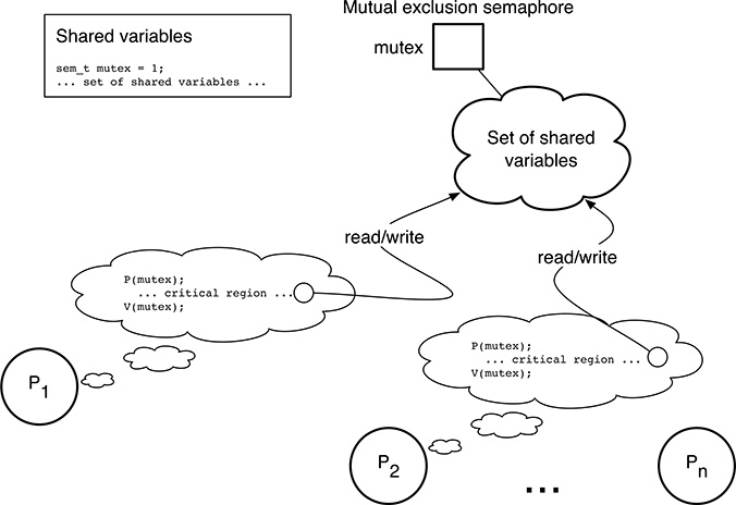
FIGURE 5.11
A semaphore can be used to enforce mutual exclusion.
When this happens, one of the processes formerly blocked on mutex will be resumed—for example P2—and will be allowed to execute the critical region code. Upon exit from the critical region, P2 will also execute V(mutex) to wake up another process, and so on, until the last process Pn exits from the critical region while no other processes are currently blocked on P(mutex).
In this case, the effect of V(mutex) is to increment the value of mutex and bring it back to 1 so that exactly one process will be allowed to enter into the critical region immediately, without being blocked, in the future.
It should also be remarked that no race conditions during semaphore manipulation are possible because the semaphore implementation must guarantee that P() and V() are executed atomically.
For what concerns the second correctness condition, it can easily be observed that the only case in which the mutual exclusion semaphore prevents a process from entering a critical region takes place when another process is already within a critical region controlled by the same semaphore. Hence, processes doing internal operations cannot prevent other processes from entering their critical regions in any way.
The behavior of semaphores with respect to the third and fourth correctness conditions depend on their implementation. In particular, both conditions can easily be fulfilled if the semaphore queuing policy is first-in first-out, so that V() always wakes up the process that has been waiting on the semaphore for the longest time. When a different queuing policy must be adopted for other reasons, for instance, to solve the unbounded priority inversion, as discussed in Chapter 15, then some processes may be subject to an indefinite wait, and this possibility must usually be excluded by other means.
Besides mutual exclusion, semaphores are also useful for condition synchronization, that is, when we want to block a process until a certain event occurs or a certain condition is fulfilled. For example, considering again the producers–consumers problem, it may be desirable to block any consumer that wants to get a data item from the shared buffer when the buffer is completely empty, instead of raising an error indication. Of course, a blocked consumer must be unblocked as soon as a producer puts a new data item into the buffer. Symmetrically, we might also want to block a consumer when it tries to put more data into a buffer that is already completely full.
In order to do this, we need one semaphore for each synchronization condition that the concurrent program must respect. In this case, we have two conditions, and hence we need two semaphores:
The semaphore
emptycounts how many empty elements there are in the buffer. Its initial value isNbecause the buffer is completely empty at the beginning. Producers perform aP(empty)before putting more data into the buffer to update the count and possibly block themselves, if there is no empty space in the buffer. After removing one data item from the buffer, consumers perform aV(empty)to either unblock one waiting producer or increment the count of empty elements.Symmetrically, the semaphore
fullcounts how many full elements there are in the buffer. Its initial value is0because there is no data in the buffer at the beginning. Consumers performP(full)before removing a data item from the buffer, and producers perform aV(full)after storing an additional data item into the buffer.
The full solution to the producers–consumers problem is shown in Figure 5.12. In summary, even if semaphores are all the same, they can be used in two very different ways, which should not be confused:
A mutual exclusion semaphore, like
mutexin the example, is used to prevent more than one process from executing within a set of critical regions pertaining to the same set of shared data. The use of a mutual exclusion semaphore is quite stereotyped: its initial value is always1, andP()andV()are placed, like brackets, around the critical regions code.A condition synchronization semaphore, such as
emptyandfullin the example, is used to ensure that certain sequences of events do or do not occur. In this particular case, we are using them to prevent a producer from storing data into a full buffer, or a consumer from getting data from an empty buffer. They are usually more difficult to use correctly because there is no stereotype to follow.
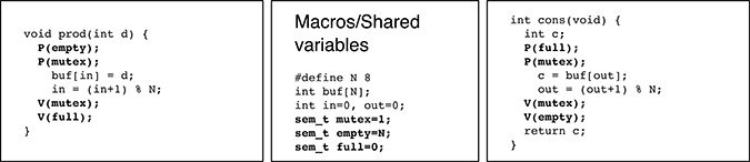
FIGURE 5.12
Producers–consumers problem solved with mutual exclusion and condition synchronization semaphores.
5.6 Monitors
As discussed in the previous section, semaphores can be defined quite easily; as we have seen, their behavior can be fully described in about one page. Their practical implementation is also very simple and efficient so that virtually all modern operating systems support them. However, semaphores are also a very low-level interprocess communication mechanism. For this reason, they are difficult to use, and even the slightest mistake in the placement of a semaphore primitive, especially P(), may completely disrupt a concurrent program.
For example, the program shown in Figure 5.13 may seem another legitimate way to solve the producers–consumers problem. Actually, it has been derived from the solution shown in Figure 5.12 by swapping the two semaphore primitives shown in boldface. After all, the program code still “makes sense” after the swap because, as programmers, we could reason in the following way:
In order to store a new data item into the shared buffer, a producer must, first of all, make sure that it is the only process allowed to access the shared buffer itself. Hence, a
P(mutex)is needed.In addition, there must be room in the buffer, that is, at least one element must be free. As discussed previously,
P(empty)updates the count of free buffer elements held in the semaphoreemptyand blocks the caller until there is at least one free element.
Unfortunately, this kind of reasoning is incorrect because the concurrent execution of the code shown in Figure 5.13 can lead to a deadlock. When a producer tries to store an element into the buffer, the following sequence of events may occur:
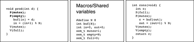
FIGURE 5.13
Semaphores may be difficult to use: even the incorrect placement of one single semaphore primitive may lead to a deadlock.
The producer succeeds in gaining exclusive access to the shared buffer by executing a
P(mutex). From this point on, the value of the semaphoremutexis zero.If the buffer is full, the value of the semaphore
emptywill be zero because its value represents the number of empty elements in the buffer. As a consequence, the execution ofP(empty)blocks the producer. It should also be noted that the producer is blocked within its critical region, that is, without releasing the mutual exclusion semaphoremutex.
After this sequence of events takes place, the only way to wake up the blocked producer is by means of a V(empty). However, by inspecting the code, it can easily be seen that the only V(empty) is at the very end of the consumer’s code. No consumer will ever be able to reach that statement because it is preceded by a critical region controlled by mutex, and the current value of mutex is zero.
In other words, the consumer will be blocked by the P(mutex) located at the beginning of the critical region itself as soon as it tries to get data item from the buffer. All the other producers will be blocked, too, as soon as they try to store data into the buffer, for the same reason.
As a side effect, the first N consumers trying to get data from the buffer will also bring the value of the semaphore full back to zero so that the following consumers will not even reach the P(mutex) because they will be blocked on P(full).
The presence of a deadlock can also be deducted in a more abstract way, for instance, by referring to the Havender/Coffman conditions presented in Chapter 4. In particular,
As soon as a producer is blocked on
P(empty)and a consumer is blocked onP(mutex), there is a circular wait in the system. In fact, the consumer waits for the producer to release the resource “empty space in the buffer,” an event represented byV(empty)in the code. Symmetrically, the consumer waits for the producer to release the resource “mutual exclusion semaphore,” an event represented byV(mutex).Both resources are subject to a mutual exclusion. The mutual exclusion semaphore, by definition, can be held by only one process at a time. Similarly, the buffer space is either empty or full, and hence may belong to either the producers or the consumers, but not to both of them at the same time.
The hold and wait condition is satisfied because both processes hold a resource—either the mutual exclusion semaphore or the ability to provide more empty buffer space—and wait for the other.
Neither resource can be preempted. Due to the way the code has been designed, the producer cannot be forced to relinquish the mutual exclusion semaphore before it gets some empty buffer space. On the other hand, the consumer cannot be forced to free some buffer space without first passing through its critical region controlled by the mutual exclusion semaphore.
To address these issues, a higher-level and more structured interprocess communication mechanism, called monitor, was proposed by Brinch Hansen [16] and Hoare [37]. It is interesting to note that, even if these proposals date back to the early ’70s, they were already based on concepts that are common nowadays and known as object-oriented programming. In its most basic form, a monitor is a composite object and contains
a set of shared data;
a set of methods that operate on them.
With respect to its components, a monitor guarantees the following two main properties:
Information hiding, because the set of shared data defined in the monitor is accessible only through the monitor methods and cannot be manipulated directly from the outside. At the same time, monitor methods are not allowed to access any other shared data. Monitor methods are not hidden and can be freely invoked from outside the monitor.
Mutual exclusion among monitor methods, that is, the monitor implementation, must guarantee that only one process will be actively executing within any monitor method at any given instant.
Both properties are relatively easy to implement in practice because monitors—unlike semaphores—are a programming language construct that must be known to, and supported by, the language compiler. For instance, mutual exclusion can be implemented by forcing a process to wait when it tries to execute a monitor method while another process is already executing within the same monitor.
This is possible because the language compiler knows that a call to a monitor method is not the same as a regular function call and can therefore handle it appropriately. In a similar way, most language compilers already have got all the information they need to enforce the information-hiding rules just discussed while they are processing the source code.
The two properties just discussed are clearly powerful enough to avoid any race condition in accessing the shared data enclosed in a monitor and are a valid substitute for mutual exclusion semaphores. However, an attentive reader would certainly remember that synchronization semaphores have an equally important role in concurrent programming and, so far, no counterpart for them has been discussed within the monitor framework.
Unsurprisingly, that counterpart does exist and takes the form of a third kind of component belonging to a monitor: the condition variables. Condition variables can be used only by the methods of the monitor they belong to, and cannot be referenced in any way from outside the monitor boundary. They are therefore hidden exactly like the monitor’s shared data. The following two primitives are defined on a condition variable c:
wait(c)blocks the invoking process and releases the monitor in a single, atomic action.signal(c)wakes up one of the processes blocked onc; it has no effect if no processes are blocked onc.
The informal reasoning behind the primitives is that, if a process starts executing a monitor method and then discovers that it cannot finish its work immediately, it invokes wait on a certain condition variable. In this way, it blocks and allows other processes to enter the monitor and perform their job.
When one of those processes, usually by inspecting the monitor’s shared data, detects that the first process can eventually continue, it calls signal on the same condition variable. The provision for multiple condition variables stems from the fact that, in a single monitor, there may be many, distinct reasons for blocking. Processes can easily be divided into groups and then awakened selectively by making them block on distinct condition variables, one for each group.
However, even if the definition of wait and signal just given may seem quite good by intuition, it is nonetheless crucial to make sure that the synchronization mechanism does not “run against” the mutual exclusion property that monitors must guarantee in any case, leading to a race condition. It turns out that, as shown in Figure 5.14, the following sequence of events involving two processes A and B may happen:
Taking for granted that the monitor is initially free—that is, no processes are executing any of its methods—process A enters the monitor by calling one of its methods, and then blocks by means of a
wait(c).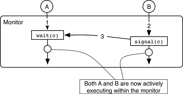
FIGURE 5.14
After await/signalsequence on a condition variable, there is a race condition that must be adequately addressed.At this point, the monitor is free again, and hence, another process B is allowed to execute within the monitor by invoking one of its methods. There is no race condition because process A is still blocked.
During its execution within the monitor, B may invoke
signal(c)to wake up process A.
After this sequence of events, both A and B are actively executing within the monitor. Hence, they are allowed to manipulate its shared data concurrently in an uncontrolled way. In other words, the mutual exclusion property of monitors has just been violated. The issue can be addressed in three different ways:
As proposed by Brinch Hansen [16], it is possible to work around the issue by constraining the placement of
signalwithin the monitor methods: in particular, if asignalis ever invoked by a monitor method, it must be its last action, and implicitly makes the executing process exit from the monitor. As already discussed before, a simple scan of the source code is enough to detect any violation of the constraint.In this way, only process A will be executing within the monitor after a
wait/signalsequence, as shown in Figure 5.15, because thesignalmust necessarily be placed right at the monitor boundary. As a consequence, process B will indeed keep running concurrently with A, but outside the monitor, so that no race condition occurs. Of course, it can also be shown that the constraint just described solves the problem in general, and not only in this specific case.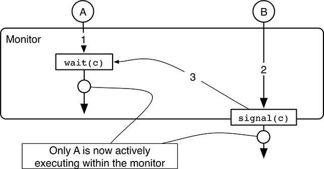
FIGURE 5.15
An appropriate constraint on the placement ofsignalin the monitor methods solves the race condition issue after await/signalsequence.The main advantage of this solution is that it is quite simple and efficient to implement. On the other hand, it leaves to the programmer the duty of designing the monitor methods so that
signalonly appears in the right places.Hoare’s approach [37] imposes no constraints at all on the placement of
signal, which can therefore appear and be invoked anywhere in monitor methods. However, the price to be paid for this added flexibility is that the semantics ofsignalbecome somewhat less intuitive because it may now block the caller.In particular, as shown in Figure 5.16, the signaling process B is blocked when it successfully wakes up the waiting process A in step 3. In this way, A is the only process actively executing in the monitor after a
wait/signalsequence and there is no race condition. Process B will be resumed when process A either exits from the monitor or waits again, as happens in step 4 of the figure.In any case, processes like B—that entered the monitor and then blocked as a consequence of a
signal—take precedence on processes that want to enter the monitor from the outside, like process C in the figure. These processes will therefore be admitted into the monitor, one at a time, only when the process actively executing in the monitor leaves or waits, and no processes are blocked due to asignal.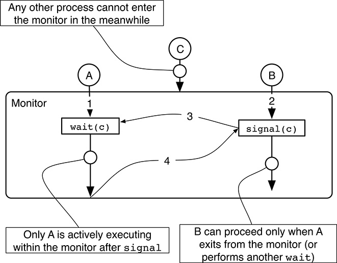
FIGURE 5.16
Another way to eliminate the race condition after await/signalsequence is to block the signaling process until the signaled one ceases execution within the monitor.The approach adopted by the POSIX standard [48] differs from the previous two in a rather significant way. Application developers must keep these differences in mind because writing code for a certain “flavor” of monitors and then executing it on another will certainly lead to unexpected results.
The reasoning behind the POSIX approach is that the process just awakened after a
wait, like process A in Figure 5.17, must acquire the monitor’s mutual exclusion lock before proceeding, whereas the signaling process (B in the figure) continues immediately. In a sense, the POSIX approach is like Hoare’s, but it solves the race condition by postponing the signaled process, instead of the signaling one.When the signaling process B eventually leaves the monitor or blocks in a
wait, one of the processes waiting to start or resume executing in the monitor is chosen for execution. This may be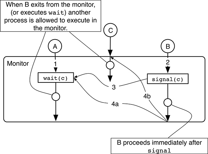
FIGURE 5.17
The POSIX approach to eliminate the race condition after await/signalsequence is to force the process just awakened from awaitto reacquire the monitor mutual exclusion lock before proceeding.one process waiting to reacquire the mutual exclusion lock after being awakened from a
wait(process A and step 4a in the figure); or,one process waiting to enter the monitor from the outside (process C and step 4b in the figure).
The most important side effect of this approach from the practical standpoint is that, when process A waits for a condition and then process B signals that the condition has been fulfilled, process A cannot be 100% sure that the condition it has been waiting for will still be true when it will eventually resume executing in the monitor. It is quite possible, in fact, that another process C was able to enter the monitor in the meantime and, by altering the monitor’s shared data, make the condition false again.
To conclude the description, Figure 5.18 shows how the producers–consumers problem can be solved by means of a Brinch Hansen monitor, that is, the simplest kind of monitor presented so far. Unlike the previous examples, this one is written in “pseudo C” because the C programming language, by itself, does not support monitors. The fake keyword monitor introduces a monitor. The monitor’s shared data and methods are syntactically grouped together by means of a pair of braces. Within the monitor, the keyword condition defines a condition variable.
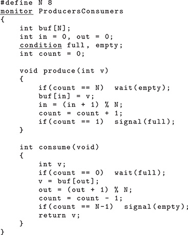
FIGURE 5.18
Producers–consumers problem solved by means of a Brinch Hansen monitor.
The main differences with respect to the semaphore-based solution of Figure 5.12 are
The mutual exclusion semaphore
mutexis no longer needed because the monitor construct already guarantees mutual exclusion among monitor methods.The two synchronization semaphores
emptyandfullhave been replaced by two condition variables with the same name. Indeed, their role is still the same: to make producers wait when the buffer is completely full, and make consumers wait when the buffer is completely empty.In the semaphore-based solution, the value of the synchronization semaphores represented the number of empty and full elements in the buffer. Since condition variables have no memory, and thus have no value at all, the monitor-based solution keeps that count in the shared variable
count.Unlike in the previous solution, all
waitprimitives are executed conditionally, that is, only when the invoking process must certainly wait. For example, the producer’swaitis preceded by anifstatement checking whethercountis equal toNor not, so thatwaitis executed only when the buffer is completely full. The same is also true forsignal, and is due to the semantics differences between the semaphore and the condition variable primitives.
5.7 Summary
In order to work together toward a common goal, processes must be able to communicate, that is, exchange information in a meaningful way. A set of shared variables is undoubtedly a very effective way to pass data from one process to another. However, if multiple processes make use of shared variables in a careless way, they will likely incur a race condition, that is, a harmful situation in which the shared variables are brought into an inconsistent state, with unpredictable results.
Given a set of shared variables, one way of solving this problem is to locate all the regions of code that make use of them and force processes to execute these critical regions one at a time, that is, in mutual exclusion. This is done by associating a sort of lock to each set of shared variables. Before entering a critical region, each process tries to acquire the lock. If the lock is unavailable, because another process holds it at the moment, the process waits until it is released. The lock is released at the end of each critical region.
The lock itself can be implemented in several different ways and at different levels of the system architecture. That is, a lock can be either hardware- or software-based. Moreover, it can be based on active or passive wait. Hardware-based locks, as the name says, rely on special CPU instructions to realize lock acquisition and release, whereas software-based locks are completely implemented with ordinary instructions.
When processes perform an active wait, they repeatedly evaluate a predicate to check whether the lock has been released or not, and consume CPU cycles doing so. On the contrary, a passive wait is implemented with the help of the operating system scheduler by moving the waiting processes into the Blocked state. This is a dedicated state of the Process State Diagram, in which processes do not compete for CPU usage and therefore do not proceed with execution.
From a practical perspective, the two most widespread ways of supporting mutual exclusion for shared data access in a real-time operating system are semaphores and, at a higher level of abstraction, monitors. Both of them are based on passive wait and are available in most modern operating systems.
Moreover, besides mutual exclusion, they can both be used for condition synchronization, that is, to establish timing constraints among processes, which are not necessarily related to mutual exclusion. For instance, a synchronization semaphore can be used to block a process until an external event of interest occurs, or until another process has concluded an activity.
Last, it should be noted that adopting a lock to govern shared data access is not the only way to proceed. Indeed, it is possible to realize shared objects that can be concurrently manipulated by multiple processes without using any lock. This will be the topic of Chapter 10.