Chapter 25. Using Financial Functions
In this chapter
Examples of Common Household Loan and Investment Functions 592
Examples of Functions for Financial Professionals 598
Examples of Depreciation Functions 603
Functions for Investment Analysis 609
Examples of Functions for Bond Investors 615
Examples of Miscellaneous Financial Functions 627
While the bulk of Excel’s financial functions are for professional financiers and investors, there are a few functions that are useful for anyone planning to use a loan to purchase a car or house. The examples in this chapter represent a small subset of the calculations possible with Excel’s financial functions.
Table 25.1 provides an alphabetical list of all of Excel 2007’s financial functions. Detailed examples of the functions are provided in the remainder of the chapter.
Table 25.1. Alphabetical List of Financial Functions
Examples of Common Household Loan and Investment Functions
While Excel is popular with banking and investment professionals, it is handy for just about anyone who deals with financial transactions. This first section of this chapter applies to anyone who is planning on buying a car or a house. With a little preplanning with Excel, you can build very simple worksheets that allow you to calculate various monthly payments for various loan amounts.
You need to keep in mind two universal rules when dealing with all financial functions:
- Make sure your time units are consistent. If you are calculating a monthly loan payment, the interest rate argument should be expressed as a monthly figure. Most interest rates are quoted as an annual figure, such as 5.5%. To convert, you divide 5.5% by 12.
- When money is changing hands, consider the direction in which money is flowing. In any transaction, some cash will be flowing toward you (positive), and some cash will be flowing away from you (negative). If you try to enter all terms as positive, you will end up with a result that is not meaningful. For example, say you want a car loan where the bank gives $20,000 at the beginning and then gives you another $377 per month.
NPER(5%/12,377,20000)would come up with an incorrect result for your problem because one of the cash flows needs to be negative. If you are considering the loan from the point of view of the customer, the formula would beNPER(5%/12,-377,20000). If you are considering the loan from the point of view of the bank, the formula would beNPER(5%/12,377,-20000).
Using PMT to Calculate the Monthly Payment on an Automobile Loan
Buying a car is one of the most exciting purchases. Whether the car is brand-new or just new to you, nothing attracts attention in your neighborhood like a new car pulling into the driveway.
Before shopping for a car, you should take a five-minute spin through Excel to calculate potential car payments. Knowing the price that will get you to the desired car payment will allow you to haggle with the sales rep from a position of knowledge.
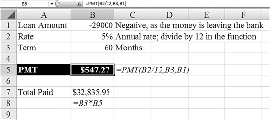
Syntax: PMT(rate,nper,pv,fv,type)
The PMT function calculates the payment for a loan based on constant payments and a constant interest rate. This function takes the following arguments:
rate—This is the interest rate for the loan. Note that interest rate is often expressed as an annual rate. If you are calculating a monthly payment, you have to divide that rate by 12.nper—This is the term, or the total number of payments for the loan.pv—This is the present value, or the loan amount; it is also known as the principal.fv—This is an optional future value, or a cash balance you want to attain after the last payment is made. For a car payment calculation, this should be0. Iffvis omitted, it is assumed to be0, that is, the future value of a loan is zero.type—This is the number0or1and indicates when payments are due. The default value of0assumes that the first payment is due after a month has elapsed. If you have to make the first payment on the day the loan is issued, you should set this value to1.
Note
The payment returned by PMT includes principal and interest but not taxes, insurance, escrow, or fees sometimes associated with loans.
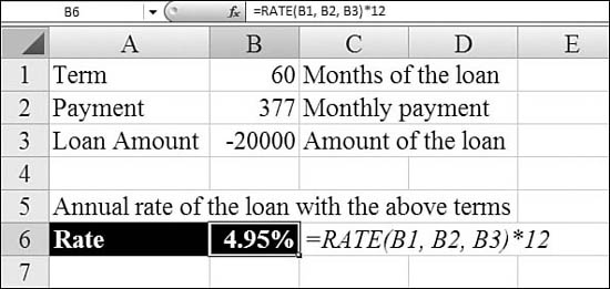
For a reality check, try multiplying the calculated payment by nper. This way, you can calculate the total of all payments over the life of the loan. In Figure 25.1, you see that a $29,000 car actually costs $32,835 in principal and interest.
Figure 25.1. PMT calculates a monthly loan payment.
Using RATE to Determine an Interest Rate
The PMT function is useful when you are considering a new loan. If you are analyzing a loan that you’ve been paying for a while, you might know the monthly payment but forget the interest rate. The RATE function can help you determine the rate.
Syntax: RATE(nper,pmt,pv,fv,type,guess)
The RATE function returns the interest rate per period of an annuity. RATE is calculated by iteration and can have zero or more solutions. If the successive results of RATE do not converge to within 0.0000001 after 20 iterations, RATE returns a #NUM! error. This function takes the following arguments:
nper—This is the total number of payment periods in an annuity.pmt—This is the payment made each period and cannot change over the life of the annuity. Typically,pmtincludes principal and interest but no other fees or taxes. Ifpmtis omitted, you must include thefvargument.pv—This is the present value—the total amount that a series of future payments is worth now.fv—This is the future value, or a cash balance you want to attain after the last payment is made. Iffvis omitted, it is assumed to be0(the future value of a loan, for example, is zero).type—This is the number0or1to indicate when payments are due. The default value of0assumes that payments are due at the end of the period. A value of1means the payments are due at beginning of each period.guess—This is your guess for what the rate will be. If you omitguess, it is assumed to be 10%. IfRATEdoes not converge, you can try different values forguess.RATEusually converges ifguessis between0and1.
Make sure you are consistent about the units you use for specifying guess and nper. If you make monthly payments on a four-year loan at 12% annual interest, you use 12% / 12 for guess and 4 × 12 for nper. If you make annual payments on the same loan, you use 12% for guess and 4 for nper.
Figure 25.2 shows how to calculate an interest rate.
Figure 25.2. Given the other terms for a loan, back into the interest rate with RATE.
Using PV to Figure Out How Much House You Can Afford
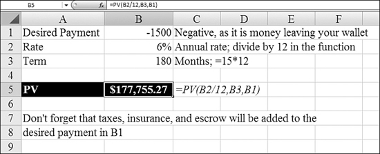
If you are looking for a monthly house payment of $1,500 with a 15-year loan at 6% annual interest rate, you can back into the loan amount by using the PV function.
Syntax: PV(rate,nper,pmt,fv,type)
The PV function returns the present value of an investment. The present value is the total amount that a series of future payments is worth now. For example, when you borrow money, the loan amount is the present value to the lender. This function takes the following arguments:
rate—This is the interest rate per period. For example, if you obtain an automobile loan at a 10% annual interest rate and make monthly payments, your interest rate per month is 10%/12, or 0.83%. You would therefore enter10%/12, or0.83%, or0.0083, into the formula asrate.nper—This is the total number of payment periods in an annuity. For example, if you get a four-year car loan and make monthly payments, your loan has 4 × 12 (or 48) periods. You would enter48into the formula fornper.pmt—This is the payment made each period and cannot change over the life of the annuity. Typically,pmtincludes principal and interest but no other fees or taxes. For example, the monthly payments on a $10,000, four-year car loan at 12% are $263.33. You would enter-263.33into the formula forpmt. Ifpmtis omitted, you must include thefvargument.fv—This is the future value, or a cash balance you want to attain after the last payment is made. Iffvis omitted, it is assumed to be0(the future value of a loan, for example, is zero). For example, if you want to save $50,000 to pay for a special project in 18 years, then $50,000 is the future value. You could then make a conservative guess at an interest rate and determine how much you must save each month. Iffvis omitted, you must include thepmtargument.type—This is the number0or1to indicate when payments are due. The default value of0assumes that payments are due at the end of the period. A value of1means the payments are due at beginning of each period.
In Figure 25.3, Cell B5 calculates the loan principal amount that would result in the desired payment, including principal and interest. You also need to budget for monthly insurance, taxes, and fees that might be a part of your monthly payment to the bank.
Figure 25.3. You use PV to calculate how much you can borrow to meet a monthly payment budget.
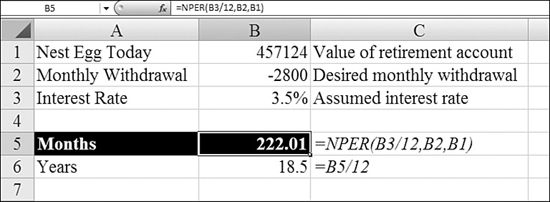
Using NPER to Estimate How Long a Nest Egg will Last
NPER stands for number of periods. If you have a 401(k) retirement account and are trying to calculate how long you can withdraw fixed monthly payments from the account, use NPER.
Syntax: NPER(rate, pmt, pv, fv, type)
The NPER function returns the number of periods for an investment, based on periodic, constant payments and a constant interest rate. This function takes the following arguments:
rate—This is the interest rate per period.pmt—This is the payment made each period; it cannot change over the life of the annuity. Typically,pmtcontains principal and interest but no other fees or taxes.pv—This is the present value, or the lump-sum amount that a series of future payments is worth right now.fv—This is the future value, or a cash balance you want to attain after the last payment is made. Iffvis omitted, it is assumed to be0(the future value of a loan, for example, is zero). If you want to leave an inheritance to your kids, you use that amount as theFV.type—This is the number0or1to indicate when payments are due. The default value of0assumes that payments are due at the end of the period. A value of1means the payments are due at beginning of each period.
In Figure 25.4, the NPER function in Cell B5 estimates how many months you can withdraw the amount in Cell B2. Note that the monthly withdrawal is negative from the point of view of the retirement account.
Figure 25.4. You use NPER to figure out how long an annuity can pay out before it ends in a zero balance.
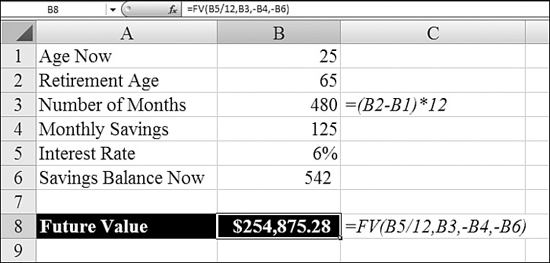
Using FV to Estimate the Future Value of a Regular Savings Plan
The future value calculation assumes that you will make regular monthly payments to a savings plan every month. It also assumes that the interest rate does not change throughout the life of the savings plan. If you are young, it is likely that you will be able to save more as your income grows later. However, using the savings calculator in Figure 25.5 helps you to realize the value of regular savings.
Figure 25.5. You can estimate the future value of a regular savings plan.
Syntax: FV(rate,nper,pmt,pv,type)
The FV function returns the future value of an investment, based on periodic, constant payments and a constant interest rate. This function takes the following arguments:
rate—This is the interest rate per period.nper—This is the total number of payment periods in an annuity.pmt—This is the payment made each period; it cannot change over the life of the annuity. Typically,pmtcontains principal and interest but no other fees or taxes. Ifpmtis omitted, you must include thepvargument.pv—This is the present value, or the lump-sum amount that a series of future payments is worth right now. Ifpvis omitted, it is assumed to be0, and you must include thepmtargument.type—This is the number0or1to indicate when payments are due. The default value of0assumes that payments are due at the end of the period. A value of1means the payments are due at beginning of each period.
For all the arguments, cash you pay out, such as deposits to savings, is represented by negative numbers; cash you receive, such as dividend checks, is represented by positive numbers.
Figure 25.5 shows how to use FV for a simple savings calculator. The formula in Cell B8 assumes that you continue making the deposit each month from Cell B4 until you retire and that interest rates remain constant. If you already have some amount in savings, you enter that in Cell B6.
Note that the FV formula uses a negative version of Cells B4 and B6. This is because these are amounts that leave your wallet and go to the bank or mutual fund.
Examples of Functions for Financial Professionals
Whereas the typical consumer is interested in the amount of his or her monthly car payment, a loan maker is interested in the month-by-month breakdown of principal and interest. Excel offers a complete cadre of functions to do these calculations.
Using PPMT to Calculate the Principal Payment for Any Month
After a bank writes a car loan, the consumer makes monthly payments. To calculate the principal portion of the payment for any period in the loan, you use PPMT. Of course, you can use a range of these formulas—one for each month—to build an amortization table.
Syntax: PPMT(rate,per,nper,pv,fv,type)
The PPMT function returns the payment on the principal for a given period for an investment, based on periodic, constant payments and a constant interest rate. This function takes the following arguments:
rate—This is the interest rate per period.per—This specifies for which period the principal payment will be returned. It must be in the range1tonper.nper—This is the total number of payment periods in an annuity.pv—This is the present value—the total amount that a series of future payments is worth now.fv—This is the future value, or a cash balance you want to attain after the last payment is made. Iffvis omitted, it is assumed to be0—that is, the future value of a loan is zero.type—This is the number0or1to indicate when payments are due. The default value of0assumes that payments are due at the end of the period. A value of1means the payments are due at beginning of each period.
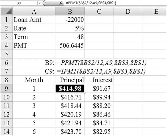
In Figure 25.6, Cell B9 calculates the principal payment for Period 1. The per argument comes from the month number in Column A. Copying the formula down for all months produces an amortization table.
Figure 25.6. Similar PPMT functions in B9:B56 calculate the monthly principal portion of the loan payment.
Note
In this example, the interest component could either be calculated with PMT–PPMT or using the IPMT function. IPMT is discussed in the next section.
Using IPMT to Calculate the Interest Portion of a Loan Payment for Any Month
Whereas the PPMT function calculates the principal payment for any month of a loan, the IPMT function calculates the interest portion of the payment. The results of IPMT are shown in Column C of Figure 25.6.
Syntax: IPMT(rate,per,nper,pv,fv,type)
The IPMT function returns the interest payment for a given period for an investment, based on periodic, constant payments and a constant interest rate. This function takes the following arguments:
rate—This is the interest rate per period.per—This is the period for which you want to find the interest and must be in the range1tonper.nper—This is the total number of payment periods in an annuity.pv—This is the present value, or the lump-sum amount that a series of future payments is worth right now.fv—This is the future value, or a cash balance you want to attain after the last payment is made.type—This is the number0or1to indicate when payments are due. The default value of0assumes that payments are due at the end of the period. A value of1means the payments are due at beginning of each period.
The IPMT function is similar to the PPMT function. Combined, they can create a simple amortization table (refer to Figure 25.6).
Note
You may encounter an old worksheet that uses ISPMT, which is the Lotus 1-2-3 version of IPMT. For details on ISPMT, see Excel Help. For new worksheets, you should use IPMT instead of ISPMT.
Using CUMIPMT to Calculate Total Interest Payments During a Time Frame
The CUMIPMT function is great for figuring out your yearly tax deduction for your mortgage interest. After specifying the typical components of a loan (that is, rate, term, amount), you specify that you want to calculate the interest for particular periods, such as Periods 6 through 18.
Syntax: CUMIPMT(rate,nper,pv,start_period,end_period,type)
The CUMIPMT function returns the cumulative interest paid on a loan between start_period and end_period. This function takes the following arguments:
rate—This is the interest rate.nper—This is the total number of payment periods.pv—This is the present value.start_period—This is the first period in the calculation. Payment periods are numbered beginning with1.end_period—This is the last period in the calculation.type—This is the number0or1to indicate when payments are due. The default value of0assumes that payments are due at the end of the period. A value of1means the payments are due at beginning of each period.
nper, start_period, end_period, and type are truncated to integers. If rate is less than or equal to 0, nper is less than or equal to 0, or pv is less than or equal to 0, CUMIPMT returns a #NUM! error. If start_period is less than 1, end_period is less than 1, or start_period is greater than end_period, CUMIPMT returns a #NUM! error. If type is any number other than 0 or 1, CUMIPMT returns a #NUM! error.
Figure 25.7 calculates the total interest paid during each year of the loan. The mildly difficult portion of the sample spreadsheet is that the number of months in the first year will likely be less than 12. Cell D12 uses =13-MONTH(B5). Cell C13 uses =D12+1. Cell D13 uses =C12+11 to calculate the last period for each year.
Figure 25.7. You use Column E to plan your tax deductions by year.
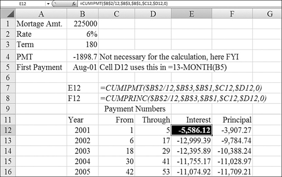
Column F of this spreadsheet uses CUMPRINC, which is discussed in the next section.
Using CUMPRINC to Calculate Total Principal Paid in Any Range of Periods
The corollary to CUMIPMT is a function to calculate the total principal paid during any range of periods of a loan: CUMPRINC.
Syntax: CUMPRINC(rate,nper,pv,start_period,end_period,type)
The CUMPRINC function returns the cumulative principal paid on a loan between start_period and end_period. This function takes the following arguments:
rate—This is the interest rate.nper—This is the total number of payment periods.pv—This is the present value.start_period—This is the first period in the calculation. Payment periods are numbered beginning with1.end_period—This is the last period in the calculation.type—This is the number0or1to indicate when payments are due. The default value of0assumes that payments are due at the end of the period. A value of1means the payments are due at beginning of each period.
nper, start_period, end_period, and type are truncated to integers. If rate is less than or equal to 0, nper is less than or equal to 0, or pv is less than or equal to 0, CUMPRINC returns a #NUM! error. If start_period is less than 1, end_period is less than 1, or start_period is greater than end_period, CUMPRINC returns a #NUM! error. If type is any number other than 0 or 1, CUMPRINC returns a #NUM! error.
Figure 25.7 shows an example of CUMPRINC.
Using EFFECT to Calculate the Effect of Compounding Period on Interest Rates
Does it really matter if your bank compounds interest daily, monthly, or quarterly? If the numbers are big enough, it can matter. The EFFECT function converts an interest rate to an effective rate, depending on how frequently the bank compounds the interest.
Syntax: EFFECT(nominal_rate,npery)
The EFFECT function returns the effective annual interest rate, given the nominal annual interest rate and the number of compounding periods per year. This function takes the following arguments:
nominal_rate—This is the nominal interest rate.npery—This is the number of compounding periods per year.nperyis truncated to an integer.
If either argument is nonnumeric, EFFECT returns a #VALUE! error. If nominal_rate is less than or equal to 0 or if npery is less than 1, EFFECT returns a #NUM! error.
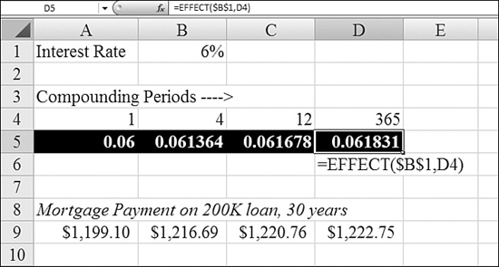
In Figure 25.8, the nominal interest rate is 6%. If the bank compounds interest once per year, the effective interest rate is still 6%, as shown in Cell A5. If interest is compounded monthly, the effective rate increases to 6.17%. Row 9 compares the monthly mortgage payment at the various effective rates. Daily compounding adds about $23 per month to a typical mortgage payment.
Figure 25.8. Row 5 shows the effective interest rates for various compounding periods. Row 9 shows the monthly payment difference.
Using NOMINAL to Convert the Effective Interest Rate to a Nominal Rate
If you need to compare two investments, one quoting a nominal rate and one quoting an effective rate, you can convert the effective rate to a nominal rate by using NOMINAL
Syntax: NOMINAL(effect_rate,npery)
The NOMINAL function returns the nominal annual interest rate, given the effective rate and the number of compounding periods per year. This function takes the following arguments:
effect_rate—This is the effective interest rate.npery—This is the number of compounding periods per year.
npery is truncated to an integer. If either argument is nonnumeric, NOMINAL returns a #VALUE! error. If effect_rate is less than or equal to 0 or if npery is less than 1, NOMINAL returns a #NUM! error.
Examples of Depreciation Functions
When a company buys a large asset, such as a piece of machinery, accounting rules specify how the asset should be expensed each year. This is called depreciation. Excel offers four common methods for calculating depreciation: straight-line, declining-balance, double-declining-balance, and sum-of-years’-digits methods.
The following terms are common to all the depreciation methods:
- Cost—This is the initial cost of the asset. For example, the machinery might cost $120,000.
- Useful life—This is how long you expect to use the asset. If you think the machinery will be used for 10 years before being replaced, the life is 10 years.
- Salvage value—This is the value of the asset at the end of the useful life. Perhaps after 10 years, you can sell the machine to a scrap dealer for $1,000 or to a trade school for $5,000. This is the salvage value.
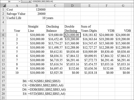
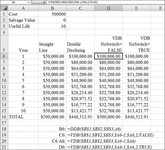
Figure 25.9 compares the four depreciation methods.
Figure 25.9. Columns B through E compare four methods of depreciation.
Using SLN to Calculate Straight-Line Depreciation
The straight-line method is the simplest depreciation method. Using this method, the value of the asset is depreciated evenly over the asset’s useful life. At the end of the useful life, the item is depreciated on the company’s books to the salvage value level.
Syntax: SLN(cost,salvage,life)
The SLN function returns the straight-line depreciation of an asset for one period. This function takes the following arguments:
cost—This is the initial cost of the asset.salvage—This is the asset’s value at the end of the depreciation period (sometimes called the salvage value of the asset).life—This is the number of periods over which the asset is being depreciated (sometimes called the useful life of the asset).
Using DB to Calculate Declining-Balance Depreciation
In the declining-balance method, depreciation happens at a constant rate. The advantage of this method is that more depreciation happens in the earlier years, providing a better tax benefit in early years.
Let’s look at a simple example. Say that a $100,000 asset is depreciated 20% in Year 1. This results in a $20,000 depreciation expense. After Year 1, the asset would be have a value of $80,000 on the books. In Year 2, the remaining balance of $80,000 is multiplied by the same 20% rate to yield a depreciation of $16,000. The depreciation in Year 3 is 20% of the remaining $64,000, or $12,800.
The trick to this method is figuring out the correct percentage to use for each year. This involves fractional exponents and a little algebra. If you use the DB function, however, you don’t have to worry about any of that. Excel calculates this rate, rounded to three decimal places, as the first step in the process. This rounding to three decimal places causes the calculation to be off by a few dollars at the end of the useful life.
For details on special handling of Year 1 and the last year, as well as the algebra behind the rate formula, see Excel Help for this function.
Syntax: DB(cost,salvage,life,period,month)
The DB function returns the depreciation of an asset for a specified period, using the fixed-declining-balance method. This function takes the following arguments:
cost—This is the initial cost of the asset.salvage—This is the value at the end of the depreciation period (sometimes called the salvage value of the asset).life—This is the number of periods over which the asset is being depreciated (sometimes called the useful life of the asset).period—This is the period for which you want to calculate the depreciation.periodmust use the same units aslife.month—This is the number of months in the first year. Ifmonthis omitted, it is assumed to be12.
Using DDB to Calculate Double-Declining-Balance Depreciation
The double-declining-balance method is a very aggressive (and legal) method for calculating depreciation. Assume that you purchased a computer. In the first year, the item might be state-of-the-art. By Year 2, it is worth far less because technology would have passed the computer by.
The name of this method reflects the fact that the depreciation rate is double the normal rate but also that the depreciation rate is applied to the declining balance of the asset’s value.
If the asset is to be depreciated over five years, the normal straight-line rate would be 20%. In the double-declining-balance method, you get to use 40% in each year. For example, the first year, depreciation on a $100,000 asset would be 40%. But in Year 2, the 40% is multiplied by the remaining asset value of $60,000. This method generates much higher depreciation in the first few years of the asset life than the other methods.
Although the name of this method contains the world double, Microsoft covered the possibility of other multipliers. There is a 150DB method that multiplies the rate by 1.5 instead of 2. To calculate 150DB, you use 1.5 as the fourth argument. If no fourth argument is supplied, the fourth argument is assumed to be 2, resulting in DDB.
Note
In many depreciation systems, you are allowed to switch from double-declining-balance to the straight-line method when the straight-line method produces a higher depreciation. To do this, you use the VDB function, which is described shortly.
Syntax: DDB(cost,salvage,life,period,factor)
The DDB function returns the depreciation of an asset for a specified period using the double-declining-balance method or some other specified method. This function takes the following arguments:
cost—This is the initial cost of the asset.salvage—This is the value at the end of the depreciation period.life—This is the number of periods over which the asset is being depreciated.period—This is the period for which you want to calculate the depreciation.periodmust use the same units as life.factor—This is the rate at which the balance declines. Iffactoris omitted, it is assumed to be2(the double-declining-balance method).
All five of these arguments must be positive numbers.
In order to allow DDB to work, you need to abandon the method at some point and switch to a straight-line method for the remaining asset value. If you attempt to use DDB for the entire life of the asset, you will not write off enough of the value.
Figure 25.10 illustrates how DDB fails to accumulate $500,000 of depreciation.
Figure 25.10. The DDB method fails to accumulate enough depreciation. You might want to use the newer VDB method, which automatically switches for you. Column D shows this method.
To overcome this problem with DDB, you can use the VDB method. The VDB function is a far more powerful function. Using VDB to calculate a double-declining-balance problem correctly is somewhat like using a sledgehammer to push in a thumbtack. VDB is covered in detail later in this chapter, but you can follow these steps to solve the current problem:
- Change the function name from
DDBtoVDB. - Because both
DDBandVDBtake the same first three arguments—cost,salvage, andlife—leave those three arguments alone. - Give
DDBa period number. Cell C6 uses the year number from Cell A6 for the period.VDBneeds a start period and an end period. ForVDB, changeA6toA6-1,A6. This is a bit strange; you are askingVDBto calculate the depreciation from the end of Year 0 to the end of Year 1. - Determine whether the DDB function is done.
factoris assumed to be2.factoris usually left off the function. IfDDBhas no fourth argument, thenVDBdoes not need a fifth argument. - To allow
VDBto switch to the straight-line method, ensure that the sixth argument isFALSE. The name of this argument isno_switch, so by specifyingFALSE, you are invoking a double negative to askVDBto switch to the straight-line method when appropriate. BecauseFALSEis the default, you can often leave off the fifth and sixth arguments withVDB.
Complete details on the more powerful uses of VDB are provided later in this chapter.
Using SYD to Calculate Sum-of-Years’-Digits Depreciation
The sum-of-years’-digits method is another accelerated depreciation system. It ensures that the value of the asset drops more in the earlier years of the asset’s life than in later years.
Say that you have an asset with a useful life of seven years. You need to add all the years from seven to one: 7 + 6 + 5 + 4 + 3 + 2 + 1 = 28. In the first year, you can write off 7 / 28 of the value. In the next year, you can write off 6 / 28. In successive years, you can write off 5 / 28, 4 / 28, 3 / 28, 2 / 28, and 1 / 28 of the depreciable value.
Syntax: SYD(cost,salvage,life,per)
The SYD function returns the sum-of-years’-digits depreciation of an asset for a specified period. This function takes the following arguments:
cost—This is the initial cost of the asset.salvage—This is the value at the end of the depreciation period (sometimes called the salvage value of the asset).life—This is the number of periods over which the asset is being depreciated (sometimes called the useful life of the asset).per—This is the period and must use the same units aslife.
Using VDB to Calculate Depreciation for Any Period
As mentioned in the discussion of the DDB function, the VDB function is newer and far more powerful than the other depreciation functions.
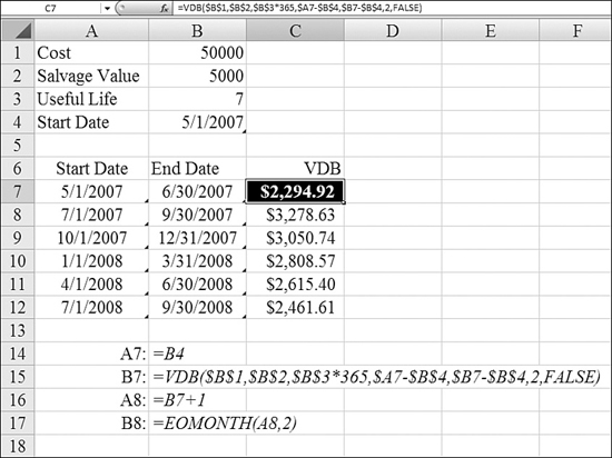
It is interesting for tax purposes to know the annual depreciation amounts. However, if you work for a public company, you have to report depreciation at least quarterly. Figure 25.11 shows an example that calculates the exact depreciation to be booked each quarter.
Figure 25.11. VDB allows you to calculate depreciation for each month or quarter.
Syntax: VDB(cost,salvage,life,start_period,end_period,factor,no_switch)
The VDB function returns the depreciation of an asset for any specified period, including partial periods, using the double-declining-balance method or some other specified method. VDB stands for variable declining balance.
The VDB function takes the following arguments:
cost—This is the initial cost of the asset.salvage—This is the value at the end of the depreciation period.life—This is the number of periods over which the asset is being depreciated. To calculate depreciation for periods smaller than a year, you multiply the number of years by 12 or even 365.start_period—This is the starting period for which you want to calculate the depreciation.start_periodmust use the same units aslife.end_period—This is the ending period for which you want to calculate the depreciation.end_periodmust use the same units aslife.factor—This is the rate at which the balance declines. Iffactoris omitted, it is assumed to be2(the double-declining-balance method). You changefactorif you do not want to use the double-declining-balance method.no_switch—This is a logical value that specifies whether to switch to straight-line depreciation when depreciation is greater than with the declining-balance calculation. If this isFALSEor omitted, Excel switches to the straight-line method when it becomes more beneficial to do so. If this value isTRUE, Excel holds on to theDDBmethod until the end oflife.
All these arguments except no_switch must be positive numbers.
To set up a schedule that shows depreciation for each quarter, you follow these steps:
- Enter the cost, salvage value, and useful life at the top of the worksheet.
- Enter the date on which the equipment is placed in service in Cell B4.
- Enter dates for the first quarter in Cells A7 and B7. The value in Cell A7 is the date the unit is placed in service. Manually figure out the last date of the quarter for Cell B7.
- Ensure that the formula for Columns A and B in each subsequent row is the same. In Cell A8, enter
=B7+1. In Cell B8, enter is=EOMONTH(A8,2). TheEOMONTHfunction reports the end of the month that falls two months after what is shown in Cell A8. Copy these formulas down as far as necessary. - To build the
VDBfunction, use the normal values for cost and salvage value. Instead of7forlife, use 7 × 365 to have the function calculate a daily depreciation rate. - For
start_period, use the date in Column A minus the date inservice. - For
end_period, use the date in Column B minus the date inservice. - If you are using the double-declining-balance method, omit the fifth and sixth arguments.
- Copy the
VDBfunction down to all your rows.
The table shown in Figure 25.11 shows the depreciation to be booked each quarter for this particular piece of machinery.
Note
If you happen to work for a French-owned company, you need to keep in mind special considerations when calculating depreciation. Read the Help topics for AMORDEGRC and AMORLINC to understand these methods that have been added to Excel to accommodate the French accounting rules.
Functions for Investment Analysis
The invention of the computer spreadsheet in 1979 enabled the rapid growth of the mergers and acquisitions business in the 1980s. Business plans can be modeled in Excel, with the resulting series of net income values discounted to determine the current value of a business. Excel offers a wide array of functions that can be used to analyze a business investment
Using the NPV Function to Determine Net Present Value
Let’s say that you have a pile of cash. You have the opportunity to invest that cash in a long-term CD that earns 4% interest. You also have the opportunity to use that cash to buy a business. The 4% is called the hurdle rate. If the business cannot return more than the 4% hurdle rate, you should probably look for another business.
You’ve analyzed the business plan and projected that the business will generate a certain series of net income over each of the next five years. You can analyze the net present value of the investment by using the NPV function.
Syntax: NPV(rate,value1,value2,...)
The NPV function calculates the net present value of an investment by using a discount rate and a series of future payments (negative values) and income (positive values). This function takes the following arguments:
rate—This is the rate of discount over the length of one period.value1,value2,...—These are 1 to 254 arguments representing the payments and income. Instead, you can refer to a range of values.value1, value2,...must be equally spaced in time and occur at the end of each period. The function uses the order ofvalue1,value2,...to interpret the order of cash flows. You need to be sure to enter your payment and income values in the correct sequence.
The NPV investment begins one period before the date of the value1 cash flow and ends with the last cash flow in the list.
Arguments of value1, value2,... are cash flows at the end of Year 1, Year 2, and so on.
In this example, if you buy a business for $50,000, this amount should not be entered as a value in the function. Instead, you should subtract the $50,000 from the result of NPV.
NPV is similar to the PV function. The primary difference between PV and NPV is that PV allows cash flows to begin either at the end or at the beginning of the period. Unlike the variable NPV cash flow values, PV cash flows must be constant throughout the investment.
NPV is also related to the IRR function. IRR is the rate for which NPV equals zero: NPV(IRR(...), ...) = 0.
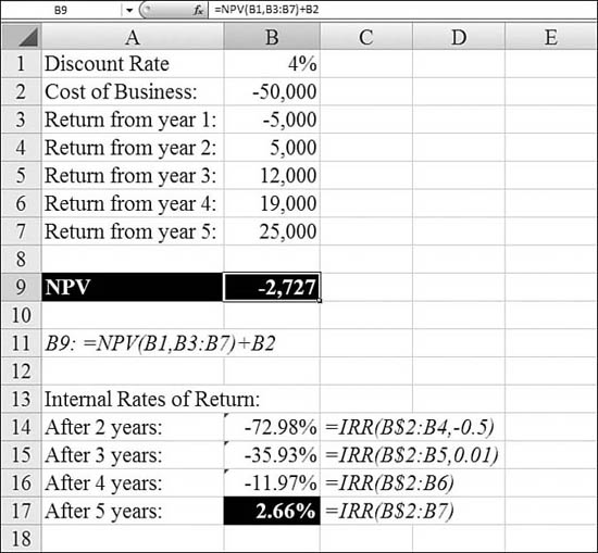
In Figure 25.12, the business will cost $50,000. The business will lose $5,000 in Year 1 and then generate $61,000 over the next four years. Based on these cash flows, NPV is negative, meaning that a CD at 4% would provide a better return.
Figure 25.12. NPV can analyze a periodic series of cash flows.
NPV requires the cash flows to occur at a regular rate. If you instead have a series of projected cash flows on varying dates, you should use XNPV instead. See the section “Using XNPV to Calculate the Net Present Value When the Payments Are Not Periodic,” later in this chapter.
Using IRR to Calculate the Return of a Series of Cash Flows
In the previous section, you used the NPV function to determine whether a business investment met or did not meet a certain desired rate of return. In Figure 25.12, NPV is negative, indicating that the business was not able to produce a 4% return after five years. If you actually want to figure out the internal rate of return, you use the IRR function.
There is one critical difference between IRR and NPV: In the NPV function, the initial investment in the business is not included in the list of arguments. In the IRR function, the initial investment in the business needs to be included as the first cash flow. Because this is money paid for the business, it should be negative.
Syntax: IRR(values,guess)
The IRR function returns the internal rate of return for a series of cash flows, represented by the numbers in values. These cash flows do not have to be even, as they would be for an annuity. However, the cash flows must occur at regular intervals, such as monthly or annually. The internal rate of return is the interest rate received for an investment, consisting of payments (negative values) and income (positive values) that occur at regular periods.
The IRR function takes the following arguments:
values—This is an array or a reference to cells that contain numbers for which you want to calculate the internal rate of return.valuesmust contain at least one positive value and one negative value to calculate the internal rate of return.IRRuses the order ofvaluesto interpret the order of cash flows. You need to be sure to enter your payment and income values in the sequence you want. If an array or a reference argument contains text, logical values, or empty cells, those values are ignored.guess—This is a number that you guess is close to the result ofIRR. Microsoft Excel uses an iterative technique for calculatingIRR. Starting withguess,IRRcycles through the calculation until the result is accurate within 0.00001%. IfIRRcan’t find a result that works after 20 tries, a#NUM!error is returned. In most cases, you do not need to provideguessfor theIRRcalculation. Ifguessis omitted, it is assumed to be0.1(that is, 10%). IfIRRgives a#NUM!error, or if the result is not close to what you expected, you can try again with a different value for guess.
IRR is closely related to NPV, the net present value function. The rate of return calculated by IRR is the interest rate corresponding to a net present value of zero. The following formula demonstrates how NPV and IRR are related: Enter = NPV(IRR(B1:B6),B1:B6) in a cell. This equals 3.60E-08 Within the accuracy of the IRR calculation, the value 3.60E-08 is effectively zero.
In Figure 25.12, the formula in Cell B17 shows that the business investment would generate a rate of return of 2.7% if analyzed over a five-year period. The arguments for this function include the initial $50,000 investment in the business as well as the net incomes from the next five years.
Similar formulas in Cells B14 and B15 return a #NUM! error. The formulas were edited to add a guess value. Based on the –12% return through four years, guess for three years was –10%.
Note
IRR fails to take into account that the money earned in Year 1 could start generating interest if invested in a CD. To calculate a rate of return including the reinvestment of profits, you use MIRR, which is described in the following section.
Using MIRR to Calculate Internal Rate of Return, Including Interest Rates
MIRR calculates a modified internal rate of return. This function assumes that cash flows from the business are reinvested at some interest rate. It also offers an argument to specify the initial interest rate of the business loan used to purchase the business.
Syntax: MIRR(values,finance_rate,reinvest_rate)
The MIRR function returns the modified internal rate of return for a series of periodic cash flows. MIRR considers both the cost of the investment and the interest received on reinvestment of cash. This function takes the following arguments:
values—This is an array or a reference to cells that contain numbers. These numbers represent a series of payments (negative values) and income (positive values) occurring at regular periods.valuesmust contain at least one positive value and one negative value to calculate the modified internal rate of return. Otherwise,MIRRreturns a#DIV/0!error. If an array or a reference argument contains text, logical values, or empty cells, those values are ignored; however, cells with the value0are included.finance_rate—This is the interest rate you pay on the money used in the cash flows.reinvest_rate—This is the interest rate you receive on the cash flows as you reinvest them.
MIRR uses the order of values to interpret the order of cash flows. You need to be sure to enter your payment and income values in the sequence you want and with the correct signs (that is, positive values for cash received, negative values for cash paid).
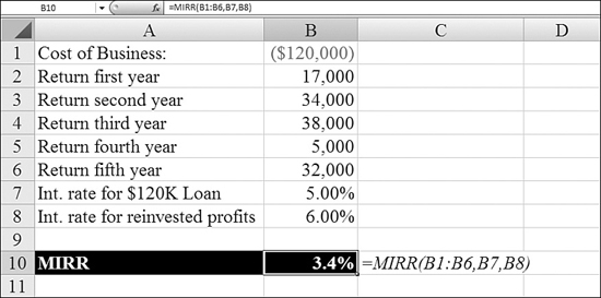
In Figure 25.13, you are analyzing a business that was started five years ago with a $120,000 loan. The business has generated profits of $17,000, $34,000, $38,000, $5,000, and $32,000. The original loan had an interest rate of 5%, and the profits were reinvested at 6%. The MIRR in Cell B10 is 3.4%. For comparison, the IRR of the same cash flows would be only 1.64%.
Figure 25.13. You can determine a modified rate of return, figuring in a financing rate and the interest rate for reinvested profits.
Using XNPV to Calculate the Net Present Value When the Payments Are Not Periodic
The previous examples assume that everything happens on the last day of each year. In reality, the business purchase date and the business sales date might occur on other days. In such a case, you use XNPV.
Syntax: XNPV(rate,values,dates)
The XNPV function returns the net present value for a schedule of cash flows that is not necessarily periodic. To calculate the net present value for a series of cash flows that is periodic, you use the NPV function. The XNPV function takes the following arguments:
rate—This is the discount rate to apply to the cash flows.values—This is a series of cash flows that corresponds to a schedule of payments indates. The first payment is optional and corresponds to a cost or payment that occurs at the beginning of the investment. If the first value is a cost or payment, it must be a negative value. All succeeding payments are discounted based on a 365-day year. The series of values must contain at least one positive value and one negative value.dates—This is a schedule of payment dates that corresponds to the cash flow payments. The first payment date indicates the beginning of the schedule of payments. All other dates must be later than this date, but they may occur in any order. Only dates are considered; any times appended to the dates are truncated.
If any argument is nonnumeric, XNPV returns a #VALUE! error. If any number in dates is not a valid date, XNPV returns a #NUM! error. If any number in dates precedes the starting date, XNPV returns a #NUM! error. If values and dates contain different numbers of values, XNPV returns a #NUM! error.
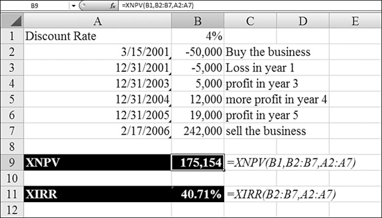
In Figure 25.14, the company was bought on March 15, 2001. The company posted no net profit in 2002. The company was sold in February 2006. The XNPV function in Row 9 shows that this deal clearly beat the 4% hurdle rate.
Figure 25.14. XNPV takes into account a series of cash flows on a series of dates. The dates don’t have to have identical periods, as in NPV.
Using XIRR to Calculate a Return Rate When Cash Flow Dates Are Not Periodic
As in the XNPV example, you can calculate an internal rate of return for a business deal where the dates don’t necessarily fall on the last day of the year. To do so, you use XIRR, an example of which is shown at the bottom of Figure 25.14.
Syntax: XIRR(values,dates,guess)
The XIRR function returns the internal rate of return for a schedule of cash flows that is not necessarily periodic. To calculate the internal rate of return for a series of periodic cash flows, you use the IRR function. This function takes the following arguments:
values—This is a series of cash flows that corresponds to a schedule of payments indates. The first payment is optional and corresponds to a cost or payment that occurs at the beginning of the investment. If the first value is a cost or payment, it must be a negative value. All succeeding payments are discounted based on a 365-day year. The series of values must contain at least one positive and one negative value.dates—This is a schedule of payment dates that corresponds to the cash flow payments. The first payment date indicates the beginning of the schedule of payments. All other dates must be later than this date, but they may occur in any order.guess—This is a number that you guess is close to the result ofXIRR.
Numbers in dates are truncated to integers. XIRR expects at least one positive cash flow and one negative cash flow; otherwise, XIRR returns a #NUM! error. If any number in dates is not a valid date, XIRR returns a #NUM! error. If any number in dates precedes the starting date, XIRR returns a #NUM! error. If values and dates contain different numbers of values, XIRR returns a #NUM! error. In most cases, you do not need to provide guess for the XIRR calculation. If it is omitted, guess is assumed to be 0.1 (that is, 10%).
XIRR is closely related to XNPV, the net present value function. The rate of return calculated by XIRR is the interest rate corresponding to XNPV = 0.
Examples of Functions for Bond Investors
A bond is an I.O.U. You lend an amount to the issuer. The issuer pays you periodic interest payments and at the maturity date of the bond returns your money. Various governments issue many bonds. Bond maturities can extend anywhere from 1 day to 30 years. Many concepts and terms apply to the bond functions.
For the following discussion, let’s assume that a city issues a 30-year municipal bond. The bond is issued on July 1, 2007. The bond’s maturity date is June 30, 2037. The city agrees to pay 5% interest semiannually.
Here is what makes bonds interesting: They can be bought and sold after the issue date. Say that 14 months have gone past. Interest rates have now risen. The bond is going to keep paying 5% interest for the next 30 years. If interest rates have moved above 5%, then a potential buyer of the bond will not want to pay $1,000 for the bond. Instead, they buyer might pay $950. Thus, there is a price paid for the bond, and there is a value of the bond at maturity.
Many bond functions ask for these arguments:
settlement—This is the day that the buyer purchases the bond. It might be the issue date but is usually after the issue date. In the preceding example, the settlement date is September 1, 2008.maturity—This is the day that the issuer will pay the face value of the bond. In the preceding example, the maturity date is June 30, 2037.rate—This is the published coupon rate for the bond. In the preceding example, it is 5%.pr—This is the price that the current buyer paid for the bond. If the bond was purchased on the issue date, the price matches the face value of the bond. If it was purchased on a later date, the price is higher or lower than the face value, depending on whether interest rates go up or down. (If interest rates go up, bond prices go down. If interest rates go down, bond prices go up).pris expressed as the price per $100 of face value. If you buy a $1,000 face-value bond for $950, the price is $95 per $100, so you enter95for thepriceargument.redemtion—This is the value of the bond on the maturity date. It is the amount the issuer will pay back to the holder of the bond. The price is expressed as the price per $100 of face value. If you buy a $1,000 face-value bond that will pay $1,000 at maturity, you enter100for theredemptionargument.frequency—This is the number of interest payments per year. For semiannual interest payments, you enter2. For quarterly payments, you enter4. For annual payments, you enter1. In Excel, these are the only threefrequencyvalues allowed.basis—This is a code used to identify the number of days in a year. The values are the same as those available in theYEARFRACfunction. See the discussion ofYEARFRACin Chapter 23, “Using Everyday Functions: Math, Date and Time, and Text Functions.” For most U.S. bonds,basisis0to indicate a 30/360 NASD calendar. For European bonds, consult Excel Help for theYIELDfunction.
Using YIELD to Calculate a Bond’s Yield
A $1,000 bond might promise to pay 5% interest. However, if you buy the bond on the secondary market for $95, the actual yield will not be 5%. As you are trying to compare various investments, comparing the yield is one way to decide between multiple investment opportunities. To do this, you can use Excel’s YIELD function.
Syntax: YIELD(settlement,maturity,rate,pr,redemption,frequency,basis)
The YIELD function returns the yield on a security that pays periodic interest. You use YIELD to calculate bond yield. This function takes the following arguments:
settlement—This is the security’s settlement date. The security settlement date is the date after the issue date when the security is traded to the buyer. Dates may be entered as text strings within quotation marks (for example,"1/30/1998","1998/01/30"), as serial numbers (for example,39156, which represents March 15, 2007), or as results of other formulas or functions (for example,DATE(2007,3,15)).maturity—This is the security’s maturity date. The maturity date is the date when the security expires.rate—This is the security’s annual coupon rate.pr—This is the security’s price per $100 face value.redemption—This is the security’s redemption value per $100 face value.frequency—This is the number of coupon payments per year. For annual payments,frequencyis1; for semiannual,frequencyis2; and for quarterly,frequencyis4.basis—This is the type of day count basis to use. It defaults to0, which is appropriate for U.S. bonds.
settlement, maturity, frequency, and basis are truncated to integers. If settlement or maturity is not a valid date, YIELD returns a #NUM! error. If rate is less than 0, YIELD returns a #NUM! error. If pr is less than or equal to 0 or if redemption is less than or equal to 0, YIELD returns a #NUM! error. If frequency is any number other than 1, 2, or 4, YIELD returns a #NUM! error. If basis is less than 0 or if basis is greater than 4, YIELD returns a #NUM! error. If settlement is greater than or equal to maturity, YIELD returns a #NUM! error.
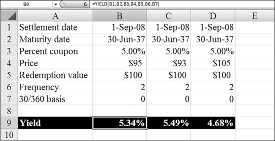
Figure 25.15 shows an example of YIELD.
Figure 25.15. You use YIELD to calculate the yield rate for a bond. In these examples, the price in Row 4 changes.
Using PRICE to Back into a Bond Price
If you know the yield for a bond, you can use PRICE to calculate the price per $100 of face value.
Syntax: PRICE(settlement,maturity,rate,yld,redemption,frequency,basis)
The PRICE function returns the price per $100 face value of a security that pays periodic interest. This function takes the following arguments:
settlement—This is the security’s settlement date. This is the date on which you purchased the bond.maturity—This is the security’s maturity date. The maturity date is the date when the security expires.rate—This is the security’s annual coupon rate.yld—This is the security’s annual yield.redemption—This is the security’s redemption value per $100 face value.frequency—This is the number of coupon payments per year. You use2for semiannual.basis—This is the type of day count basis to use. You use0for U.S. bonds.
settlement, maturity, frequency, and basis are truncated to integers. If settlement or maturity is not a valid date, PRICE returns a #NUM! error. If yld is less than 0 or if rate is less than 0, PRICE returns a #NUM! error. If redemption is less than or equal to 0, PRICE returns a #NUM! error. If frequency is any number other than 1, 2, or 4, PRICE returns a #NUM! error. If basis is less than 0 or if basis is greater than 4, PRICE returns a #NUM! error. If settlement is greater than or equal to maturity, PRICE returns a #NUM! error.
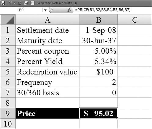
In Figure 25.16, the yield for the bond exceeds the coupon rate. This indicates that the price will be less than $100.
Figure 25.16. If you know the yield, you can back into the price by using the PRICE function.
When a bond is sold on the secondary market, it is often sold in between interest payments. Each interest payment date is called a coupon date. You analyze days until the next coupon date by using the COUP functions.
A whole series of COUP functions analyze the coupon period. The functions can tell you the previous coupon date, the next coupon date, how many days since the previous coupon date, and how many days until the next coupon date:
COUPDAYS—This returns the number of days in this coupon period.COUPDAYBS—This returns the number of days from the beginning of the coupon period until the settlement date. TheBSin the function name stands for from beginning to settlement.COUPDAYSNC—This returns the number of days from the settlement until the next coupon date.NCstands for next coupon.COUPPCD—This returns the date of the previous coupon date.COUPNCD—This returns the date of the next coupon date.COUPNUM—This returns the number of coupon dates left until maturity.
All the COUP functions require the same four arguments: settlement, maturity, frequency, and basis. For an explanation of these arguments, see the sections on YIELD and PRICE.
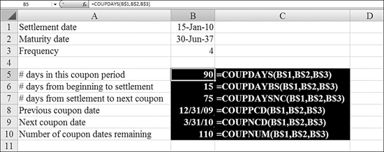
Figure 25.17 shows these coupon functions for a particular security.
Figure 25.17. You can analyze what portion of a coupon period has gone past at the settlement date for the bond.
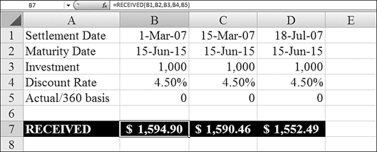
Using RECEIVED to Calculate Total Cash Generated from a Bond Investment
When you buy a bond, your settlement date is probably between two coupon dates. Unless you are buying the bond on the issue date, you receive less than the complete number of interest payments. To calculate the total future cash flows from a bond from the day you buy it until the maturity date, you use the RECEIVED function.
Syntax: RECEIVED(settlement,maturity,investment,discount,basis)
The RECEIVED function returns the amount received at maturity for a fully invested security. This function takes the following arguments:
settlement—This is the security’s settlement date. This is the date on which you purchased the security.maturity—This is the security’s maturity date. The maturity date is the date when the security expires.investment—This is the amount invested in the security.discount—This is the security’s discount rate.basis—This is the type of day count basis to use. You use0for U.S. bonds.
settlement, maturity, and basis are truncated to integers. If settlement or maturity is not a valid date, RECEIVED returns a #NUM! error. If investment is less than or equal to 0 or if discount is less than or equal to 0, RECEIVED returns a #NUM! error. If basis is less than 0 or if basis is greater than or equal to 4, RECEIVED returns a #NUM! error. If settlement is greater than or equal to maturity, RECEIVED returns a #NUM! error.
In Figure 25.18, Columns B, C, and D show the total received for a bond purchased on various dates. The function takes into account the days to the next coupon date.
Figure 25.18. In the 15 days between Cells B1 and C1, you lose $4 in interest.
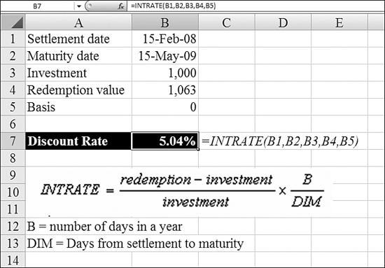
Using INTRATE to Back into the Coupon Interest Rate
If you have a fully invested bond and know what it will pay on maturity, you can use Excel’s INTRATE function to back into the interest rate.
Syntax: INTRATE(settlement,maturity,investment,redemption,basis)
The INTRATE function returns the interest rate for a fully invested security. This function takes the following arguments:
settlement—This is the security’s settlement date.maturity—This is the security’s maturity date.investment—This is the amount invested in the security.redemption—This is the amount to be received at maturity.basis—This is the type of day count basis to use. You use0for U.S. bonds.
settlement, maturity, and basis are truncated to integers. If settlement or maturity is not a valid date, INTRATE returns a #NUM! error. If investment is less than or equal to 0 or if redemption is less than or equal to 0, INTRATE returns a #NUM! error. If basis is less than 0 or if basis is greater than 4, INTRATE returns a #NUM! error. If settlement is greater than or equal to maturity, INTRATE returns a #NUM! error.
INTRATE calculates (Redemption value – Investment) / Investment and multiplies this by (Number of days in year / Days from settlement to maturity).
In Figure 25.19, Excel uses INTRATE to back into the interest rate that the bond is paying.
Figure 25.19. The INTRATE function can be used to derive the underlying interest rate for the bond.
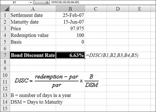
Using DISC to Back Into the Discount Rate
If you have a security and know the price, you can back into the discount rate by using DISC.
Syntax: DISC(settlement,maturity,pr,redemption,basis)
The DISC function returns the discount rate for a security. It takes the following arguments:
settlement—This is the security’s settlement date.maturity—This is the security’s maturity date. The maturity date is the date when the security expires.pr—This is the security’s price per $100 face value.redemption—This is the security’s redemption value per $100 face value.basis—This is the day count basis. You use0for U.S. bonds.
settlement, maturity, and basis are truncated to integers. If settlement or maturity is not a valid date, DISC returns a #NUM! error. If pr is less than or equal to 0 or if redemption is less than or equal to 0, DISC returns a #NUM! error. If basis is less than 0 or if basis is greater than 4, DISC returns a #NUM! error. If settlement is greater than or equal to maturity, DISC returns a #NUM! error.
DISC calculates (Redemption value – Par value) / Par value and multiplies this by (Number of days in year / Days from settlement to maturity).
In Figure 25.20, Excel uses DISC to back into the discount rate.
Figure 25.20. The DISC function can be used to derive the underlying discount rate for a bond.
Handling Bonds with an Odd Number of Days in the First or Last Period
Excel provides four functions—ODDFPRICE, ODDFYIELD, ODDLPRICE, and ODDLYIELD—to handle the special case in which a bond has a short or long first or last period. This period has more or fewer days than all the other periods and is called an odd period. For an explanation of the arguments to these functions, see the information on the PRICE and YIELD functions, earlier in this chapter.
Syntax: ODDFPRICE(settlement,maturity,issue,first_coupon,rate,yld,redemption,frequency,basis) AND ODDFYIELD(settlement,maturity,issue,first_coupon,rate,pr,redemption,frequency,basis)
The ODDF functions handle cases in which the first period has an odd number of days. These are ODDFPRICE and ODDFYIELD. Each function has the extra argument first_coupon, which specifies the date for the odd first period.
Syntax: ODDLPRICE(settlement,maturity,last_interest,rate,yld,redemption,frequency,basis) AND ODDLYIELD(settlement,maturity,last_interest,rate,pr,redemption,frequency,basis)
The ODDL functions handle cases in which the last period has an odd number of days. These are ODDLPRICE and ODDLYIELD. These functions have the extra argument last_interest, which is the date of the final interest payment before maturity. Using this date, Excel can determine the length of the time for the last period.
Using PRICEMAT and YIELDMAT to Calculate Price and Yield for Zero-Coupon Bonds
A zero-coupon bond does not pay interest on the coupon dates. All interest is paid at maturity. Excel provides PRICEMAT and YIELDMAT to calculate price and yield for these securities. Figure 25.21 illustrates both of these functions.
Figure 25.21. YIELDMAT and PRICEMAT calculate bonds for which the interest is not paid until maturity.
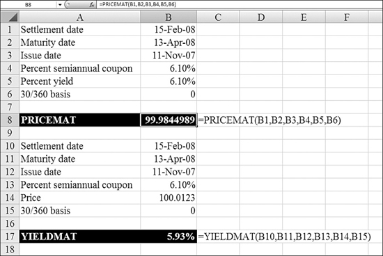
Syntax: PRICEMAT(settlement_date,maturity_date,issue_date,rate_at_date_of_issue,annual_yield,day_basis)
The PRICEMAT function returns the price per $100 face value of a security that pays interest at maturity.
Syntax: YIELDMAT(settlement_date,maturity_date,issue_date,rate_at_date_of_issue,=price_per_$100_of_face_value,day_basis)
The YIELDMAT function returns the annual yield of a security that pays interest at maturity.
Using PRICEDISC and YIELDDISC to Calculate Discount Bonds
Excel provides PRICEDISC and YIELDDISC for calculating discounted bonds. Figure 25.22 illustrates these functions.
Figure 25.22. YIELDDISC and PRICEDISC calculate discounted bonds.
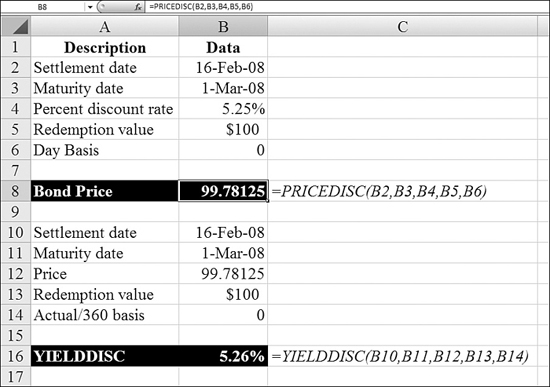
Syntax: PRICEDISC(settlement_date,maturity_date,discount_rate,redemption_value_per_$100,day_basis)
The PRICEDISC function returns the price per $100 face value of a discounted security.
Syntax: YIELDDISC(settlement_date,maturity_date,price_per_$100_face_value,redemption_value_per_$100_of_face_value,day_basis)
The YIELDDISC function returns the annual yield for a discounted security.
Calculating T-Bills
Treasury bills (T-bills) are a popular short-term investment. Backed by the U.S. government, they are considered one of the safest investments, although they offer a slightly lower interest rate than other types of investments.
The Federal Reserve uses a strange method for advertising the yield on T-bills: The Fed compares the total interest to the final value paid on maturity. This is backward from every other bond yield.
For example, say that you pay $98.7 for a T-bill that will pay $100 on maturity 13 weeks later. The Fed expresses the yield by comparing the $1.30 in interest to the $100 final value. Every other bond yield compares the $1.30 in interest to the $98.70 invested.
The Excel TBILL functions allow you to easily compare T-bills and regular bonds. Figure 25.23 illustrates the three T-bill functions.
Figure 25.23. TBILLEQ and the other TBILL functions deal with the irregularities of T-bill investing.
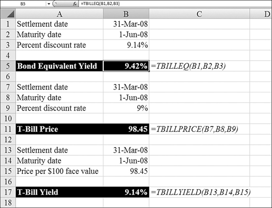
Syntax: TBILLEQ(settlement_date,maturity_date,discount_rate)
The TBILLEQ function returns the bond-equivalent yield for a T-bill.
Syntax: TBILLPRICE(settlement_date,maturity_date,discount_rate)
The TBILLPRICE function returns the price per $100 face value for a T-bill.
Syntax: TBILLYIELD(settlement_date,maturity_date,price_per_$100_face_value)
The TBILLYIELD function returns the yield for a T-bill.
Using ACCRINT or ACCINTM to Calculate Accrued Interest
If you are the original buyer of a bond and you buy that bond after the issue date, the bond will have earned some accrued interest during that gap. As the original buyer of the bond, you generally pay this interest back to the issuer when you take possession of the bond. This basically simplifies accounting for the issuer, which can issue identical payments at the next coupon date without having to worry about dozens of different settlement dates.
The ACCINT function calculates this accrued interest.
Syntax: ACCRINT(issue,first_interest,settlement,rate,par,frequency,basis)
The ACCRINT function returns the accrued interest for a security that pays periodic interest. This function takes the following arguments:
issue—This is the security’s issue date.first_interest—This is the security’s first interest date.settlement—This is the security’s settlement date. The security settlement date is the date after the issue date when the security is traded to the buyer. TheACCRINTfunction calculates the interest that would have been earned between the issue date and the settlement date.rate—This is the security’s annual coupon rate.par—This is the security’s par value. If you omitpar,ACCRINTuses $1,000.frequency—This is the number of coupon payments per year.basis—This is the type of day count basis to use. You use0for U.S. bonds
If issue is greater than or equal to settlement, ACCRINT returns a #NUM! error.
Figure 25.24 demonstrates how the accrued interest changes when the gap between the issue date and settlement date extends.
Figure 25.24. As the original buyer of the bond, you owe the accrued interest to the issuer.
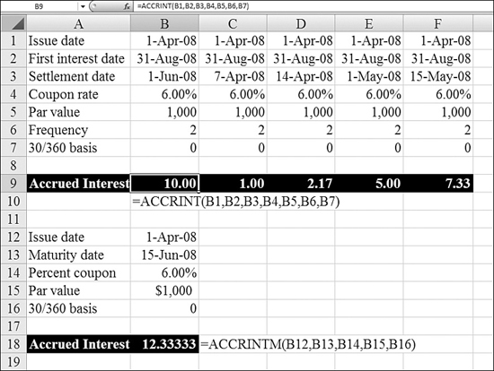
Note
The ACCINTM function calculates accrued interest for zero-coupon bonds (see Row 18 in Figure 25.24).
Using DURATION to Understand Price Volatility
Duration is a measurement, in years, of how long it takes for the price of a bond to be repaid by its cash flows. This measurement is not relevant for zero-coupon bonds because with a zero coupon bond, the duration is simultaneous with the maturity date.
Say that you have a 20-year bond with a 9% yield that pays interest twice a year. It might take about six years of interest payments before you earn back the original purchase price of the bond.
Duration is constantly changing. Immediately after a coupon date, the duration goes up slightly because the interest payment is no longer counted as a future cash flow. However, over the life of the bond, the duration gets progressively shorter, until the duration date corresponds with the maturity date. Duration is important because the higher the duration, the higher the price volatility for the security.
When Excel calculates a duration, using the DURATION function, it uses the method designed by Frederick Macaulay in the 1930s. This method multiplies the present value of each cash flow by the time it is received. Those values are summed and divided by the total price for the security.
Excel also has a modified duration function, MDURATION. This function calculates the duration if the yield would increase by 1% point. In Figure 25.25, the duration for the 9% yield is 5.99 years. The MDURATION return is 5.736 years. This is the duration if the yield would change from 9% to 10%. The difference between the duration and modified duration is an indicator of a bond price’s volatility.
Figure 25.25. DURATION indicates how many years it will take to earn back the security’s purchase price. MDURATION shows the change in duration if the yield were to increase by 1%.

Syntax: DURATION(settlement_date,maturity_date,coupon_rate,yield_rate,frequency,basis)
The DURATION function returns the Macaulay duration for an assumed par value of $100. Duration is defined as the weighted average of the present value of the cash flows and is used as a measure of a bond price’s response to changes in yield.
Syntax: MDURATION(settlement_date,maturity_date,coupon_rate,yield_rate,frequency,basis)
The MDURATION function returns the modified duration for a security with an assumed par value of $100.
Examples of Miscellaneous Financial Functions
Excel offers a few other financial functions that may be useful if you are dealing with ancient historical data. On April 9, 2001, all U.S. stock markets were forced to start trading securities in dollars and cents instead of dollars and fractions. The United States was the last nation using the fractional system, which was an 18th-century system.
In the fractional system, a stock price may have been reported in the newspaper as 5![]() , which is roughly equivalent to $5.63. However, a common system in brokerage houses was to record this as 5.5, with the .5 indicating
, which is roughly equivalent to $5.63. However, a common system in brokerage houses was to record this as 5.5, with the .5 indicating ![]() . In an alternate system, prices were recorded in 16ths, with, for example, 1.03 meaning
. In an alternate system, prices were recorded in 16ths, with, for example, 1.03 meaning ![]() .
.
Figure 25.26 shows an example of the functions Excel provides for converting between fractional numbers and decimal numbers.
Figure 25.26. You can convert old-style security fractional numbers to regular decimals and back by using DOLLARFR and DOLLARDE.
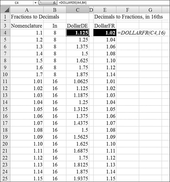
Using DOLLARDE to Convert to Decimals
If you encounter an old worksheet that uses fractional prices, you can convert them to decimals by using DOLLARDE. You must specify the price in the nomenclature of the system and specify whether the number after the decimal point is in 8ths, 16ths, or 32nds.
Syntax: DOLLARDE(fractional_dollar,fraction)
The DOLLARDE function converts a dollar price expressed as a fraction into a dollar price expressed as a decimal number. You use DOLLARDE to convert fractional dollar numbers, such as securities prices, to decimal numbers.
fractional_dollar—This is a number expressed as a fraction.fraction—This is the integer to use in the denominator of the fraction.
Syntax: DOLLARFR(decimal_dollar,fraction)
The DOLLARFR function converts a dollar price expressed as a decimal number into a dollar price expressed as a fraction.
Using FVSCHEDULE to Calculate the Future Value for a Variable Scheduled Interest Rate
The FV function discussed at the beginning of this chapter assumes a constant interest rate. If you have a loan agreement that specifies a variable interest rate for future years, you can calculate the future value based on the scheduled interest rate. To do so, you use the FVSCHEDULE function.
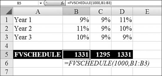
Syntax: FVSCHEDULE(principal,schedule)
The FVSCHEDULE function returns the future value of an initial principal after applying a series of compound interest rates. You use FVSCHEDULE to calculate the future value of an investment with a variable or adjustable rate. This function takes the following arguments:
principal—This is the present value.schedule—This is an array of interest rates to apply.
The values in schedule can be numbers or blank cells; any other value produces a #VALUE! error for FVSCHEDULE. Blank cells are taken as zeros (that is, no interest).
Figure 25.27 shows three examples of variable interest rates.
Figure 25.27. Calculating a future value for a series of scheduled future interest rates by using FVSCHEDULE.