
For the time-bounded classes, we show a weaker result.
Theorem 1.23
Proof
A nondecreasing function f(n) is called superpolynomial if
for all i ≥ 1. For instance, the exponential function 2n is superpolynomial, and the functions ![]() , for k > 1, are also superpolynomial.
, for k > 1, are also superpolynomial.
Corollary 1.24
Proof
Corollary 1.25
It follows that ![]() and
and ![]() .
.
The above time and space hierarchy theorems can also be extended to nondeterministic time- and space-bounded complexity classes. The proofs, however, are more involved, because acceptance and rejection in NTMs are not symmetric. We only list the simpler results on nondeterministic space-bounded complexity classes, which can be proved by a straightforward diagonalization. For the nondeterministic time hierarchy, see Exercise 1.28.
Theorem 1.26
Proof
In addition to the diagonalization technique, some other proof techniques for separating complexity classes are known. For instance, the following result separating the classes ![]() and PSPACE is based on a closure property of PSPACE that does not hold for
and PSPACE is based on a closure property of PSPACE that does not hold for ![]() . Unfortunately, this type of indirect proof techniques is not able to resolve the question of whether
. Unfortunately, this type of indirect proof techniques is not able to resolve the question of whether ![]() or
or ![]() .
.
Theorem 1.27
Proof
1.7 Simulation
We study, in this section, the relationship between deterministic and nondeterministic complexity classes, as well as the relationship between time- and space-bounded complexity classes. We show several different simulations of nondeterministic machines by deterministic ones.
Theorem 1.28
Proof
Corollary 1.29
Next we consider the space complexity of the deterministic simulation of nondeterministic space-bounded machines.
Theorem 1.30
Proof
Corollary 1.31
For any complexity class ![]() , let
, let ![]() (or, co-
(or, co-![]() ) denote the class of complements of sets in
) denote the class of complements of sets in ![]() , that is,
, that is, ![]() , where
, where ![]() , and Σ is the smallest alphabet such that
, and Σ is the smallest alphabet such that ![]() . One of the differences between deterministic and nondeterministic complexity classes is that deterministic classes are closed under complementation, but this is not known to be true for nondeterministic classes. For instance, it is not known whether NP = coNP. The following theorem shows that for most interesting nondeterministic space-bounded classes
. One of the differences between deterministic and nondeterministic complexity classes is that deterministic classes are closed under complementation, but this is not known to be true for nondeterministic classes. For instance, it is not known whether NP = coNP. The following theorem shows that for most interesting nondeterministic space-bounded classes ![]() ,
, ![]() .
.
Theorem 1.32
Proof
Recall that in the formal language theory, a language L is called context-sensitive if there exists a grammar G generatingthe language L with the right-hand side of each grammar rule in G being at least as long as its left-hand side. A well-known characterization for the context-sensitive languages is that the context-sensitive languages are exactly the class ![]() .
.
Corollary 1.33
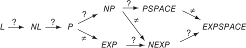
Figure 1.7 Inclusive relations among the complexity classes. We write L to denote LOGSPACE and NL to denote NLOGSPACE. The label  means the proper inclusion. The label ? means the inclusion is not known to be proper.
The above results, together with the ones proved in the last section, are the best we know about the relationship among time/space-bounded deterministic/nondeterministic complexity classes. Many other important relations are not known. We summarize in Figure 1.7 the known relations among the most familiar complexity classes. More complexity classes between P and PSPACE will be introduced in Chapters 3, 8, 9, and 10. Complexity classes between LOGSPACE and P will be introduced in Chapter 6.
Exercises
1.1 Let ![]() be q natural numbers, and Σ be an alphabet of r symbols. Show that there exist q strings
be q natural numbers, and Σ be an alphabet of r symbols. Show that there exist q strings ![]() over Σ, of lengths
over Σ, of lengths ![]() , respectively, which form an alphabet if and only if
, respectively, which form an alphabet if and only if ![]() .
.
- 1.2 a. Let c ≥ 0 be a constant. Prove that no pairing function
 exists such that for all
  ,
,  .
. - b. Prove that there exists a pairing function
 such that (i) for any
  ,
,  , (ii) it is polynomial-time computable, and (iii) its inverse function is polynomial-time computable (if
  , then
  ).
). - c. Let
 be defined by
  . Prove that f is one–one, onto, polynomial-time computable (with respect to the binary representations of natural numbers) and that
  is polynomial-time computable. (Therefore, f is an efficient pairing function on natural numbers.)
1.3 There are two cities T and F. The residents of city T always tell the truth and the residents of city F always lie. The two cities are very close. Their residents visit each other very often. When you walk in city T you may meet a person who came from city F, and vice versa. Now, suppose that you are in one of the two cities and you want to find out which city you are in. Also suppose that you are allowed to ask a person on the street for only one YES/NO question. What question should you ask? [Hint: You may first design a Boolean function f of two variables, the resident and the city, for your need, and then find a question corresponding to f.]
1.4 How many Boolean functions of n variables are there?
1.5 Assume that f is a Boolean function of more than two variables. Prove that for any minterm p of ![]() , there exists a minterm of f containing p as a subterm.
, there exists a minterm of f containing p as a subterm.
1.6 Design a multi-tape DTM M to accept the language ![]() . Show the computation paths of M on inputs
. Show the computation paths of M on inputs ![]() and
and ![]() .
.
1.7 Design a multi-tape NTM M to accept the language ![]() for some
for some ![]() . Show the computation tree of M on input
. Show the computation tree of M on input ![]() . What is the time complexity of M?
. What is the time complexity of M?
1.8 Show that the problem of Example 1.2 can be solved by a DTM in polynomial time.
1.9 Give formal definitions of the configurations and the computation of a k-tape DTM.
1.10 Assume that M is a three-tape DTM using tape alphabet ![]() . Consider the one-tape DTM M1 that simulates M as described in Theorem 1.16. Describe explicitly the part of the transition function of M1 that moves the tape head from left to right to collect the information of the current tape symbols scanned by M.
. Consider the one-tape DTM M1 that simulates M as described in Theorem 1.16. Describe explicitly the part of the transition function of M1 that moves the tape head from left to right to collect the information of the current tape symbols scanned by M.
1.11 Let ![]() is an undirected graph,
is an undirected graph, ![]() are connected}. Design an NTM M that accepts set C in space
are connected}. Design an NTM M that accepts set C in space ![]() . Can you find a DTM accepting C in space
. Can you find a DTM accepting C in space ![]() ? (Assume that
? (Assume that ![]() . Then, the input to the machine M is
. Then, the input to the machine M is ![]() , where
, where ![]() if
if ![]() and
and ![]() otherwise.)
otherwise.)
1.12 Prove that any finite set of strings belongs to ![]() .
.
1.13 Estimate an upper bound for the number of possible computation histories ![]() in the proof of Proposition 1.13.
in the proof of Proposition 1.13.
1.14 A random access machine (RAM) is a machine model for computing integer functions. The memories of a RAM M consists of a one-way read-only input tape, a one-way write-only output tape, and an infinite number of registers named ![]() Each square of the input and output tapes and each register can store an integer of an arbitrary size. Let
Each square of the input and output tapes and each register can store an integer of an arbitrary size. Let ![]() denote the content of the register Ri. An instruction of a RAM may access a register Ri to get its content
denote the content of the register Ri. An instruction of a RAM may access a register Ri to get its content ![]() or it may access the register
or it may access the register ![]() by the indirect addressing scheme. Each instruction has an integer label, beginning from 1. A RAM begins the computation on instruction with label 1 and halts when it reaches an empty instruction. The following table lists the instruction types of a RAM.
by the indirect addressing scheme. Each instruction has an integer label, beginning from 1. A RAM begins the computation on instruction with label 1 and halts when it reaches an empty instruction. The following table lists the instruction types of a RAM.
In the above table, we only listed the arguments in the direct addressing scheme. It can be changed to indirect addressing scheme by changing the argument Ri to ![]() . For instance, add
. For instance, add![]() means to write
means to write ![]() to Rk. Each instruction can also use a constant argument i instead of Rj. For instance, copy
to Rk. Each instruction can also use a constant argument i instead of Rj. For instance, copy![]() means to write integer i to the register
means to write integer i to the register ![]() .
.
- a. Design a RAM that reads inputs
 and outputs 1 if
  for some
  and outputs 0 otherwise (cf. Example 1.7).
 - b. Show that for any TM M, there is a RAM M′ that computes the same function as M. (You need to first specify how to encode tape symbols of the TM M by integers.)
- c. Show that for any RAM M, there is a TM M′ that computes the same function as M (with the integer n encoded by the string an).
1.15 In this exercise, we consider the complexity of RAMs. There are two possible ways of defining the computational time of a RAM M on input x. The uniform time measure counts each instruction as taking one unit of time and so the total runtime of M on x is the number of times M executes an instruction. The logarithmic time measure counts, for each instruction, the number of bits of the arguments involved. For instance, the total time to execute the instruction mult![]() is
is ![]() . The total runtime of M on x, in the logarithmic time measure, is the sum of the instruction time over all instructions executed by M on input x. Use both the uniform and the logarithmic time measures to analyze the simulations of parts (b) and (c) of Exercise 1.14. In particular, show that the notion of polynomial-time computability is equivalent between TMs and RAMs with respect to the logarithmic time measure.
. The total runtime of M on x, in the logarithmic time measure, is the sum of the instruction time over all instructions executed by M on input x. Use both the uniform and the logarithmic time measures to analyze the simulations of parts (b) and (c) of Exercise 1.14. In particular, show that the notion of polynomial-time computability is equivalent between TMs and RAMs with respect to the logarithmic time measure.
1.16 Suppose that a TM is allowed to have infinitely many tapes. Does this increase its computation power as far as the class of computable sets is concerned?
1.17 Prove Blum's speed-up theorem. That is, find a function ![]() such that for any DTM M1 computing f there exists another DTM M2 computing f with
such that for any DTM M1 computing f there exists another DTM M2 computing f with ![]() for infinitely many
for infinitely many ![]() .
.
1.18 Prove that if c > 1, then for any ε > 0,
1.19 Prove Theorem 1.15.
1.20 Prove that if f(n) is an integer function such that (i) ![]() and (ii) f, regarded as a function mapping an to
and (ii) f, regarded as a function mapping an to ![]() , is computable in deterministic time
, is computable in deterministic time ![]() , then f is fully time constructible. [Hint: Use the linear speed-up of Proposition 1.13 to compute the function f in less than f(n) moves, with the output
, then f is fully time constructible. [Hint: Use the linear speed-up of Proposition 1.13 to compute the function f in less than f(n) moves, with the output ![]() compressed.]
compressed.]
1.21 Prove that if f is fully space constructible and f is not a constant function, then ![]() . (We say
. (We say ![]() if there exists a constant c > 0 such that
if there exists a constant c > 0 such that ![]() for almost all n ≥ 0.)
for almost all n ≥ 0.)
1.22 Prove that ![]() and
and ![]() are fully space constructible.
are fully space constructible.
1.23 Prove that the question of determining whether a given TM halts in time p(n) for some polynomial function p is undecidable.
1.24 Prove that for any one-worktape DTM M that uses space s(n), there is a one-worktape DTM M′ with ![]() such that it uses space s(n) and its tape head never moves to the left of its starting square.
such that it uses space s(n) and its tape head never moves to the left of its starting square.
1.25 Recall that ![]() (k iterations of
(k iterations of ![]() on n)
on n) ![]() . Let k > 0 and t2 be a fully time-constructible function. Assume that
. Let k > 0 and t2 be a fully time-constructible function. Assume that
Prove that there exists a language L that is accepted by a k-tape DTM in time ![]() but not by any k-tape DTM in time
but not by any k-tape DTM in time ![]() .
.
1.26 Prove that ![]() .
.
- 1.27 a. Prove Theorem 1.26 (cf. Theorems 1.30 and 1.32).
- b. Prove that for any integer k ≥ 1 and any rational ε > 0,
 .
.
- 1.28 a. Prove that
 .
. - b. Prove that
 for any k ≥ 1.
1.29 Prove that ![]() and
and ![]() .
.
1.30 A set A is called a tally set if ![]() for some symbol a. A set A is called a sparse set if there exists a polynomial function p such that
for some symbol a. A set A is called a sparse set if there exists a polynomial function p such that ![]() for all n ≥ 1. Prove that the following are equivalent:
for all n ≥ 1. Prove that the following are equivalent:
 .
.- All tally sets in NP are actually in P.
- All sparse sets in NP are actually in P. (Note: The above implies that if
 then
then  .)
.)
1.31 (BUSY BEAVER) In this exercise, we show the existence of an r.e., nonrecursive set without using the diagonalization technique. For each TM M, we let ![]() denote the length of the codes for M. We consider only one-tape TMs with a fixed alphabet
denote the length of the codes for M. We consider only one-tape TMs with a fixed alphabet ![]() . Let
. Let ![]() and
and ![]() . That is, f(x) is the size of the minimum TM that outputs x on the input λ, and g(m) is the least x that is not printable by any TM M of size
. That is, f(x) is the size of the minimum TM that outputs x on the input λ, and g(m) is the least x that is not printable by any TM M of size ![]() on the input λ. It is clear that both f and g are total functions.
on the input λ. It is clear that both f and g are total functions.
- Prove that neither f nor g is a recursive function.
- Define
 . Apply part (a) above to show that A is r.e. but is not recursive.
1.32 (BUSY BEAVER, time-bounded version) In this exercise, we apply the busy beaver technique to show the existence of a set computable in exponential time but not in polynomial time.
- Let
 be the least
  that is not printable by any TM M of size
  on input λ in time
  . It is easy to see that
  , and hence, g is polynomial length bounded. Prove that
  is computable in time
  but is not computable in time polynomial in
  .
. - Can you modify part (a) above to prove the existence of a function that is computable in subexponential time (e.g.,
 ) but is not polynomial-time computable?
1.33 Assume that an NTM computes the characteristic function χA of a set A in polynomial time, in the sense of Definition 1.8. What can you infer about the complexity of set A?
1.34 In the proof of Theorem 1.30, the predicate reach was solved by a deterministic recursive algorithm. Convert it to a nonrecursive algorithm for the predicate reach that only uses space ![]() .
.
1.35 What is wrong if we use the following simpler algorithm to compute Nk in the proof of Theorem 1.32?
For each k, to compute Nk, we generate each configurationone by one and, for each one, nondeterministically verify whether
(by machine M1), and increments the counter for Nk by one if
holds.
1.36 In this exercise, we study the notion of computability of real numbers. First, for each ![]() , we let
, we let ![]() denote its binary expansion, and for each
denote its binary expansion, and for each ![]() , let
, let ![]() if x ≥ 0, and
if x ≥ 0, and ![]() if x < 0. An integer
if x < 0. An integer ![]() is represented as
is represented as ![]() . A rational number
. A rational number ![]() with
with ![]() , b ≠ 0, and
, b ≠ 0, and ![]() has a unique representation over alphabet
has a unique representation over alphabet ![]() :
: ![]() . We write
. We write ![]() (
(![]() and
and ![]() ) to denote both the set of natural numbers (integers and rational numbers, respectively) and the set of their representations. We say a real number x is Cauchy computable if there exist two computable functions
) to denote both the set of natural numbers (integers and rational numbers, respectively) and the set of their representations. We say a real number x is Cauchy computable if there exist two computable functions ![]() and
and ![]() satisfying the property Cf,m:
satisfying the property Cf,m: ![]() . A real number x is Dedekind computable if the set
. A real number x is Dedekind computable if the set ![]() is computable. A real number x is binary computable if there is a computable function
is computable. A real number x is binary computable if there is a computable function ![]() , with the property
, with the property ![]() for all n > 0, such that
for all n > 0, such that
where ![]() if x ≥ 0 and
if x ≥ 0 and ![]() if x < 0. (The function bx is not unique for some x, but notice that for such x, both the functions bx are computable.) A real number x is Turing computable if there exists a DTM M that on the empty input prints a binary expansion of x (i.e., it prints the string
if x < 0. (The function bx is not unique for some x, but notice that for such x, both the functions bx are computable.) A real number x is Turing computable if there exists a DTM M that on the empty input prints a binary expansion of x (i.e., it prints the string ![]() followed by the binary point and then followed by the infinite string
followed by the binary point and then followed by the infinite string ![]() ).
).
Prove that the above four notions of computability of real numbers are equivalent. That is, prove that a real number x is Cauchy computable if and only if it is Dedekind computable if and only if it is binary computable if and only if it is Turing computable.
1.37 In this exercise, we study the computational complexity of a real number. We define a real number x to be polynomial-time Cauchy computable if there exist a polynomial-time computable function ![]() and a polynomial function
and a polynomial function ![]() , satisfying Cf,m, where f being polynomial-time computable means that f(n) is computable by a DTM in time p(n) for some polynomial p (i.e., the input n is written in the unary form). We say x is polynomial-time Dedekind computable if Lx is in P. We say x is polynomial-time binary computable if bx, restricted to inputs n > 0, is polynomial-time computable, assuming that the inputs n are written in the unary form.
, satisfying Cf,m, where f being polynomial-time computable means that f(n) is computable by a DTM in time p(n) for some polynomial p (i.e., the input n is written in the unary form). We say x is polynomial-time Dedekind computable if Lx is in P. We say x is polynomial-time binary computable if bx, restricted to inputs n > 0, is polynomial-time computable, assuming that the inputs n are written in the unary form.
Prove that the above three notions of polynomial-time computability of real numbers are not equivalent. That is, let PC (PD, and Pb) denote the class of polynomial-time Cauchy (Dedekind and binary, respectively) computable real numbers. Prove that ![]() .
.
Historical Notes
McMillan's theorem is well known in coding theory; see, for example, Roman (1992). TMs were first defined by Turing (1936, 1937). The equivalent variations of TMs, the notion of computability, and the Church–Turing Thesis are the main topics of recursive function theory; see, for example, Rogers (1967) and Soare (1987). Kleene (1979) contains an interesting personal account of the history. The complexity theory based on TMs was developed by Hartmanis and Stearns (1965), Stearns, Hartmanis, and Lewis (1965) and Lewis, Stearns, and Hartmanis (1965). The tape compression theorem, the linear speed-up theorem, the tape-reduction simulations (Corollaries 1.14–1.16) and the time and space hierarchy theorems are from these works. A machine-independent complexity theory has been established by Blum (1967). Blum's speed-up theorem is from there. Cook (1973a) first established the nondeterministic time hierarchy. Seiferas (1977a, 1977b) contain further studies on the hierarchy theorems for nondeterministic machines. The indirect separation result, Theorem 1.27, is from Book (1974a). The identification of P as the class of feasible problems was first suggested by Cobham (1964) and Edmonds (1965). Theorem 1.30 is from Savitch (1970). Theorem 1.32 was independently proved by Immerman (1988) and Szelepcsényi (1988). Hopcroft et al. (1977) and Paul et al. (1983) contain separation results between ![]() ,
, ![]() , and
, and ![]() . Context-sensitive languages and grammars are major topics in formal language theory; see, for example, Hopcroft and Ullman (1979).
. Context-sensitive languages and grammars are major topics in formal language theory; see, for example, Hopcroft and Ullman (1979).
RAMs were first studied in Shepherdson and Sturgis (1963) and Elgot and Robinson (1964). The improvements over the time hierarchy theorem, including Exercises 1.25 and 1.26, can be found in Paul (1979) and Fürer (1984). Exercise 1.30 is an application of the Translation Lemma of Book (1974b); see Hartmanis et al. (1983). The busy beaver problems (Exercises 1.31 and 1.32) are related to the notion of the Kolmogorov complexity of finite strings. The arguments based on the Kolmogorov complexity avoids the direct use of diagonalization. See Daley (1980) for discussions on the busy beaver proof technique, and Li and Vitányi (1997) for a complete treatment of the Kolmogorov complexity. Computable real numbers were first studied by Turing (1936) and Rice (1954). Polynomial-time computable real numbers were studied in Ko and Friedman (1982) and Ko (1991a).