
This method has the following property.
Theorem 11.24
To show this theorem, let us first prove a few lemmas.
Lemma 11.25
Proof
Lemma 11.26
Proof
Lemma 11.27
Proof
Now, we are ready to prove Theorem 11.24.
Proof of Theorem 11.24. Part (1) holds trivially. We next show part (2).
Assume that a is an assignment for ![]() such that aX, the restriction of a on X, is δ-far from every satisfying assignment for Ψ for some
such that aX, the restriction of a on X, is δ-far from every satisfying assignment for Ψ for some ![]() . (If Ψ is not satisfiable, let δ be any constant
. (If Ψ is not satisfiable, let δ be any constant ![]() .)
.)
Case 1. L is δ-far from every linear function or Q is δ-far from every linear function.
In this case, the assignment testing proof system rejects, by Theorem 11.21, at step (1) with probability at least δ.
Case 2. L is δ-close to a linear function with coefficient vector c, and Q is δ-close to a linear function with coefficient matrix C.
Subcase 2.1. ![]() for some
for some ![]() .
.
Then, by Lemma 11.26, the assignment testing proof system rejects at step (2) with probability at least ![]() .
.
Subcase 2.2. ![]() .
.
If c does not satisfy ![]() , then by Lemma 11.27, the assignment testing proof system rejects at step (3) with probability at least
, then by Lemma 11.27, the assignment testing proof system rejects at step (3) with probability at least ![]() .
.
Next, assume that c satisfies ![]() . Then, cX, the assignment c restricted to X, is a satisfying assignment of Ψ. As aX is δ-far from every satisfying assignment of Ψ, aX is δ-far from cX. Note that L is δ-close to the linear function with coefficient vector c. By Lemma 11.22,
. Then, cX, the assignment c restricted to X, is a satisfying assignment of Ψ. As aX is δ-far from every satisfying assignment of Ψ, aX is δ-far from cX. Note that L is δ-close to the linear function with coefficient vector c. By Lemma 11.22, ![]() with probability
with probability ![]() . Therefore, with probability
. Therefore, with probability ![]() , the assignment testing proof system checks atstep (4) whether
, the assignment testing proof system checks atstep (4) whether ![]() for some
for some ![]() , and rejects with probability at least
, and rejects with probability at least ![]() .
.
From the above case analysis, we see that the assignment testing proof system must reject with probability at least ![]() . Note that if Ψ is not satisfiable, then the assignment testing proof system must reject in step (1), (2), or (3), with probability at least δ.
. Note that if Ψ is not satisfiable, then the assignment testing proof system must reject in step (1), (2), or (3), with probability at least δ. ![]()
![]()
Finally, we note that we can convert the tests in steps (1)–(4) in the assignment testing proof system into constraints over variables in ![]() and variables corresponding to the values of L and Q. For instance, suppose that
and variables corresponding to the values of L and Q. For instance, suppose that ![]() are variables for assignment a,
are variables for assignment a, ![]() are variables for L, and
are variables for L, and ![]() are variables for Q. Then, we can generate the following constraints for step (1):
are variables for Q. Then, we can generate the following constraints for step (1):
and the following constraints for step (2):
for all ![]() and all
and all ![]() .
.
Note that each run of the assignment testing proof system consists of five tests, two for step (1) and one for each of steps (2)—(4). Each test can be converted to a quadratic equation over up to 6 variables, We can further combine these five constraints into a single constraint. That is, assume the constraints of step (1) are Ck,j, ![]() , and
, and ![]() , and the constraints of step
, and the constraints of step ![]() ,
, ![]() , are Ci,j for
, are Ci,j for ![]() . Then, we generate
. Then, we generate ![]() constraints, each of the form
constraints, each of the form ![]() . It can be checked that such a constraint constains at most 19 variables. It is not hard to see that such a constraint c on 19 variables
. It can be checked that such a constraint constains at most 19 variables. It is not hard to see that such a constraint c on 19 variables ![]() can be transformed into a constant set of binary constraints
can be transformed into a constant set of binary constraints ![]() over a fixed alphabet Σ0, with possibly a constant number of additional variables
over a fixed alphabet Σ0, with possibly a constant number of additional variables ![]() , that has the following property: If an assignment σ on variables in X does not satisfy c then, for all assignments
, that has the following property: If an assignment σ on variables in X does not satisfy c then, for all assignments ![]() on variables in Y, at least one of the constraints ci,
on variables in Y, at least one of the constraints ci, ![]() , is not satisfied by
, is not satisfied by ![]() (cf. the proof of part
(cf. the proof of part ![]() of Proposition 11.5). It means that the rejection probability
of Proposition 11.5). It means that the rejection probability ![]() of the assignment testing proof system becomes unsatisfying ratio
of the assignment testing proof system becomes unsatisfying ratio ![]() for the set of binary constraints generated from the tests.
for the set of binary constraints generated from the tests.
With this conversion, we obtain, from the assignment testing proof system, an algorithm of assignment tester, that transforms a Boolean circuit Ψ on variables X to a constraint graph ![]() , with
, with ![]() and
and ![]() such that
such that
- If
 SAT
SAT , then there exists an assignment σ to all vertices in Y such that
  ; and
; and - Ifa is δ-far from any satisfying assignment of Ψ for some
 , then
  for all assignments σ on vertices in Y, where ε > 0 is an absolute constant.
This completes the construction of the assignment tester.
11.3 Probabilistic Checking and Inapproximability
We studied in Section 2.5 the approximation versions of NP-hard optimization problems. Recall that for an optimization problem Π and a real number r > 1, the problem r-APPROX-Π is its approximation version with the approximation ratio r. We have seen that some NP-hard optimization problems, such as the traveling salesman problem (TSP), are so hard to approximate that, for all approximation ratios r > 1, their approximation versions remain to be NP-hard. We also showed that for some problems, there is a threshold ![]() such that its approximation version is polynomial-time solvable with respect to the approximation ratio r0, and it is NP-hard with respect to any approximation ratio r,
such that its approximation version is polynomial-time solvable with respect to the approximation ratio r0, and it is NP-hard with respect to any approximation ratio r, ![]() . The TSP with the cost function satisfying the triangle inequality is a candidate for such a problem. In this and the next sections, we apply the PCP characterization of NP to show more inapproximability results of these two types. We first establish the NP-hardness of two prototype problems: the approximation to the maximum satisfiability problem and the approximation to the maximum clique problem. In the next section, other NP-hard approximation problems will be proved by reductions from these two problems.
. The TSP with the cost function satisfying the triangle inequality is a candidate for such a problem. In this and the next sections, we apply the PCP characterization of NP to show more inapproximability results of these two types. We first establish the NP-hardness of two prototype problems: the approximation to the maximum satisfiability problem and the approximation to the maximum clique problem. In the next section, other NP-hard approximation problems will be proved by reductions from these two problems.
For any 3-CNF Boolean formula F, let c(F) be the number of clauses in F and ![]() the maximum number of clauses that can be satisfied by a Boolean assignment on the variables of F. The maximum satisfiability problem is to find the value
the maximum number of clauses that can be satisfied by a Boolean assignment on the variables of F. The maximum satisfiability problem is to find the value ![]() for a given 3-CNF Boolean formula F. Its approximation version is formulated as follows:
for a given 3-CNF Boolean formula F. Its approximation version is formulated as follows:
r-APPROX-3SAT: Given a 3-CNF formula F, find an assignment to the Boolean variables of F that satisfies at leastclauses.
In order to prove the NP-hardness of approximation problems like r-APPROX-3SAT, we first generalize the notion of NP-complete decision problems. Let A,B be languages over some fixed alphabet Σ such that ![]() . We write (A,B) to denote the partial decision problem that asks, for a given input
. We write (A,B) to denote the partial decision problem that asks, for a given input ![]() , whether
, whether ![]() or
or ![]() . (It is called a partial decision problem because for inputs
. (It is called a partial decision problem because for inputs ![]() , we do not care what the decision is. It is sometimes also called a promise problem because it is promised that the input will be either in A or in B.) The notions of complexity and completeness of decision problems can be extended to partial decision problems in a natural way. In particular, we say the partial problem (A,B) is in the complexity class
, we do not care what the decision is. It is sometimes also called a promise problem because it is promised that the input will be either in A or in B.) The notions of complexity and completeness of decision problems can be extended to partial decision problems in a natural way. In particular, we say the partial problem (A,B) is in the complexity class ![]() if there exists a decision problem
if there exists a decision problem ![]() such that
such that ![]() and
and ![]() . Assume that
. Assume that ![]() . Then, we say the problem (A,B) is polynomial-time (many-one) reducible to the problem (C,D) and write
. Then, we say the problem (A,B) is polynomial-time (many-one) reducible to the problem (C,D) and write ![]() , if there exists a polynomial-time computable function f such that for any
, if there exists a polynomial-time computable function f such that for any ![]() ,
,
In Example 11.1, we introduced the ![]() GAP-3SAT problem. Using the notation we just introduced, we can see that
GAP-3SAT problem. Using the notation we just introduced, we can see that ![]() GAP-3SAT is just the partial problem (SAT, r-UNSAT), where SAT is the set of all satisfiable 3-CNF formulas and r-UNSAT is the set of all 3-CNF formulas with
GAP-3SAT is just the partial problem (SAT, r-UNSAT), where SAT is the set of all satisfiable 3-CNF formulas and r-UNSAT is the set of all 3-CNF formulas with![]() . From Proposition 11.5 and the PCP theorem, we get the following result.
. From Proposition 11.5 and the PCP theorem, we get the following result.
Theorem 11.28
Corollary 11.29
Proof
It is not hard to see that there exists a polynomial-time algorithm that solves the problem 2-APPROX-3SAT (see Exercise 11.16). Thus the above result establishes that there exists a threshold ![]() such that r0-APPROX-3SAT is in P and r-APPROX-3SAT is NP-hard for all
such that r0-APPROX-3SAT is in P and r-APPROX-3SAT is NP-hard for all ![]() . Indeed, the threshold r0 has been proven to be equal to 8/7 by Hastad (1997) and Karloff and Zwick (1997).
. Indeed, the threshold r0 has been proven to be equal to 8/7 by Hastad (1997) and Karloff and Zwick (1997).
Next we consider the maximum clique problem. For any graph G, we let ![]() denote the size of its maximum clique.
denote the size of its maximum clique.
r-APPROX-CLIQUE: Given a graph, find a clique Q of G whose size is at least
.
We are going to show that for all r > 1, the problem r-APPROX-CLIQUE is NP-hard. Similar to the problem r-APPROX-3SAT, we will establish this result through the NP-completeness of a partial decision problem. Recall that ![]() . Let s-NOCLIQUE
. Let s-NOCLIQUE ![]() .
.
Theorem 11.30
Proof
Corollary 11.31
The above result shows that the maximum clique ![]() of a graph G cannot be approximated within any constant factor of
of a graph G cannot be approximated within any constant factor of ![]() , if
, if ![]() . Can we approximate
. Can we approximate ![]() within a factor of a small function of the size of G, for instance,
within a factor of a small function of the size of G, for instance, ![]() (i.e., can we find a clique of size guaranteed to be at least
(i.e., can we find a clique of size guaranteed to be at least ![]() )? The answer is still no, unless
)? The answer is still no, unless ![]() . Indeed, if we explore the construction of the PCP system for NP further, we could actually show that the maximum clique problem is not approximable in polynomial time with ratio
. Indeed, if we explore the construction of the PCP system for NP further, we could actually show that the maximum clique problem is not approximable in polynomial time with ratio ![]() for any ε > 0, unless
for any ε > 0, unless ![]() (Håstad, 1996). On the positive side, the current best heuristic algorithm for approximating
(Håstad, 1996). On the positive side, the current best heuristic algorithm for approximating ![]() can only achieve the approximation ratio
can only achieve the approximation ratio ![]() (Boppana and Halldórsson, 1992).
(Boppana and Halldórsson, 1992).
11.4 More NP-Hard Approximation Problems
Starting from the problems s-APPROX-3SAT and s-APPROX-CLIQUE, we can use reductions to prove new approximation problems to be NP-hard. These reductions are often based on strong forms of reductions between the corresponding decision problems. There are several types of strong reductions in literature.In this section, we introduce a special type of strong reduction, called the L-reduction, among optimization problems that can be used to establish the NP-hardness of the corresponding approximation problems.
Recall from Section 2.5 that for a given instance x of an optimization problem Π, there are a number of solutions y to x, each with a value ![]() (or, v(y), if the problem Π is clear from the context). The problem Π is to find, for a given input x, a solution y with the maximum (or the minimum) v(y). We let
(or, v(y), if the problem Π is clear from the context). The problem Π is to find, for a given input x, a solution y with the maximum (or the minimum) v(y). We let ![]() (or, simply,
(or, simply, ![]() ) denote the value of the optimum solutions to x for problem Π.
) denote the value of the optimum solutions to x for problem Π.
An L-reduction from an optimization problem Π to another optimization problem Γ, denoted by ![]() , consists of two polynomial-time computable functions h and g and two constants
, consists of two polynomial-time computable functions h and g and two constants ![]() , which satisfy the following properties:
, which satisfy the following properties:
- L1 For any instance x of Π, h(x) is an instance of Γ such that
 .
. - L2 For any solution y of instance h(x) with value
 , g(y) is a solution of x with value
  such that

We show the L-reduction in Figure 11.1, where y∗ denotes the optimum solution to h(x) and z∗ denotes the optimum solution to x.
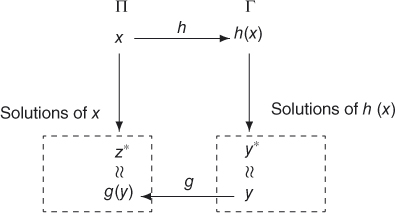
Figure 11.1 The L-reduction.
It is easy to see that the L-reduction is transitive and, hence, is really a reducibility relation.
Proposition 11.32
Proof
For any integer b > 0, consider the following two optimization problems:
VC-b: Given a graph G in which every vertex has degree at most b, find the minimum vertex cover of G.IS-b: Given a graph G in which every vertex has degree at most b, find the maximum independent set of vertices of G.