Unfortunately, the results of Theorem 7.22 are not known to hold for d-self-reducible sets, because the depth-first pruning procedure does not work for d-self-reducing trees. However, we can still prove that, assuming , NP-complete sets are not sparse by a different pruning technique on the d-self-reducing trees of SAT.
Theorem 7.24
Proof
Remark
7.4 Density of EXP-Complete Sets
In view of the difficulty of the Berman–Hartmanis isomorphism conjecture, researchers have studied the conjecture with respect to other complexity classes in order to gain more insight into this problem. One of the much studied direction is the exponential-time version of the Berman–Hartmanis conjecture. Oneof the advantages of studying the conjecture with respect to EXP is that we can perform diagonalization in EXP against all sets in P. Indeed, in this and the next sections, we will show some stronger results that reveal interesting structures of EXP-complete sets that are not known for NP-complete sets.
We begin with the notion of p-immune sets that is motivated by the notion of immune sets in recursion theory. Recall that a set A is called immune if A does not have an infinite r.e. subset. Thus, an r.e. set whose complement is immune (such a set is called a simple set) has, intuitively, very high density (because it intersects with every co-r.e. set) and, hence, cannot be -complete for r.e. sets. Here, we argue that P-immune sets cannot be -complete for EXP.
Definition 7.25
There is an interesting characterization of bi-immune sets in terms of -reductions. We say a function is finite-to-one if for every , the set is finite.
Proposition 7.26
Proof
A generalization of the bi-immune set based on the above characterization is the strongly bi-immune set.
Definition 7.27
One might suspect that the requirement of almost one-to-oneness is too strong for any set to have this property. Interestingly, there are even sparse sets that are strongly bi-immune. We divide the construction of such a set into two steps.
Theorem 7.28
Proof
Corollary 7.29
Proof
From the above theorem, we obtain a stronger version of Theorem 7.24 on EXP. First, we give some more definition.
Definition 7.30
Obviously a sparse set has subexponential density. A set of density also has subexponential density. We note that if a set B has subexponential density and via an almost one-to-one reduction, then A also has subexponential density (Exercise 7.9). Thus, let B be any EXP-complete set and A a strongly bi-immune set in EXP. We can see that B does not have subexponential density because otherwise both A and have subexponential density, which is impossible. (Note that if B is -complete for EXP, then so is .)
Corollary 7.31
7.5 One-Way Functions and Isomorphism in EXP
In Section 7.3, we mentioned that one of the difficulties of proving the Berman–Hartmanis conjecture (for the class NP) is that it is a strong statement that implies . Another difficulty involves with the notion of one-way functions. Recall that a function is a (weak) one-way function if it is one-to-one, polynomially honest, polynomial-time computable but not polynomial-time invertible (see Section 4.2). Suppose such a one-way function f exists. Then, consider the set . It is easy to see that A is NP-complete. However, it is difficult to see how it is p-isomorphic to SAT: the isomorphism function, if exists, must be different from the function f, for otherwise we could use it to compute in polynomial time. (If f is a strong one-way function, then the isomorphism function would be substantially different from f, as we cannot compute even a small fraction of ). Thus, if one-way functions exist, then it seems possible to construct a set A that is NP-complete but not p-isomorphic to SAT. On the other hand, if one-way functions do not exist, then all one-to-one polynomially honest reduction functions are polynomial-time invertible, and so the Berman–Hartmanis conjecture seems more plausible.
Based on this idea and the study of the notion of k-creative sets, Joseph and Young proposed a new conjecture:
Joseph–Young Conjecture: The Berman–Hartmanis conjecture is true if and only if one-way functions do not exist.
Although this conjecture has some interesting ideas behind it, there is not much progress in this direction yet (but see Exercises 7.12 and 7.13 for the study on k-creative sets). In this section, instead, we investigate the isomorphism conjecture on EXP-complete sets and its relation with the existence of one-way functions.
We first generalize the notion of paddable sets to weakly paddable sets and use this notion to show that all EXP-complete sets are equivalent under the -reduction.
Definition 7.32
In Section 7.2, we showed that a paddable NP-complete set must be p-isomorphic to SAT. The following is its analog for weakly paddable sets.
Lemma 7.33
Proof
Thus, it follows immediately that all -complete sets in EXP are equivalent under , if all EXP-complete sets are known to be weakly paddable.
Lemma 7.34
Proof
Combining Lemmas 7.33 and 7.34, we get the following theorem.
Theorem 7.35
From Theorem 7.4, we know that if two sets A and B are equivalent under length-increasing polynomial-time invertible reductions, then they are p-isomorphic. Observe that if one-way functions do not exist, then a -reduction is also a -reduction. So, we get the following corollary.
Corollary 7.36
In the following, we show that the converse of the above corollary holds for sets that are -complete for EXP.
In order to prove this result, we need one-way functions that are length-increasing. The following lemma shows that this requirement is not too strong.
For convenience, we will define sets A and B over the alphabet . Before we construct sets A and B, we first define two one-way functions f0 and f1 and discuss their properties.
Let be a length-increasing one-way function. Extend f to on as follows:
Case 1. If , then .
Case 2. If for some , then .
Case 3. If x contains more than one 's, then .
Now, define and . It is clear that both f0 and f1 are length-increasing one-way functions on .
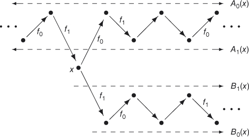
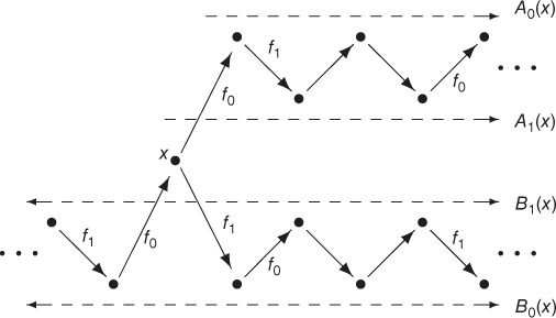
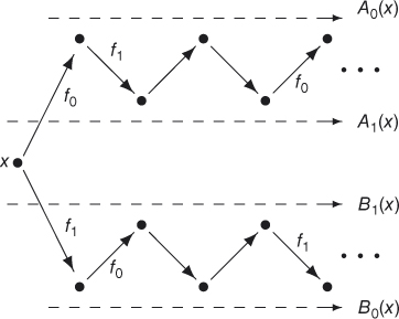
Next, define, for each , four sets as follows:
Each of these sets is called a chain (because f0 and f1 are length-increasing). We call the A-chain for x and the B-chain for x. (Note thatthe A-chain for x could be the B-chain for some other string y.) We list their basic properties in the following (see Figures 7.3–7.5).
For any , .
If x ends with 0, then x is the smallest element in and is the smallest element of .
If x ends with 1, then x is the smallest element in and is the smallest element of .
If x ends with , then x is the smallest element of both and ,
is the smallest element of
, and is the smallest element
of .
Let be an enumeration of polynomial-time TMs, ϕi the function computed by Mi, and pi a polynomial
bound of the runtime of Mi. Then the following holds:

 .
.