
Chapter 7
Polynomial-Time Isomorphism
Two decision problems are said to be polynomial-time isomorphic if there is a membership-preserving one-to-one correspondence between the instances of the two problems, which is both polynomial-time computable and polynomial-time invertible. Thus, this is a stronger notion than the notion of equivalence under the polynomial-time many-one reductions. It has, however, been observed that many reductions constructed between natural NP-complete problems are not only many-one reductions but can also be easily converted to polynomial-time isomorphisms. This observation leads to the question of whether two NP-complete problems must be polynomial-time isomorphic. Indeed, if this is the case then, within a polynomial factor, all NP-complete problems are actually identical and any heuristics for a single NP-complete problem works for all of them. In this chapter, we study this question and the related questions about the isomorphism of EXP-complete and P-complete problems.
7.1 Polynomial-Time Isomorphism
Let us start with a simple example.
Example 7.1
We now give the formal definition of the notion of polynomial-time isomorphism.
Definition 7.2
Clearly, if ![]() and
and ![]() , then
, then ![]() . For example, in addition to the problems IS and CLIQUE of Example 7.1, consider a third problem, VC:
. For example, in addition to the problems IS and CLIQUE of Example 7.1, consider a third problem, VC:
VERTEX COVER (VC): Given a graph G and an integer k > 0, determine whether G has a vertex cover of size at most k.
It is clear that a subset A of vertices is an independent set of a graph ![]() if and only if the complement set
if and only if the complement set ![]() is a vertex cover of G. This suggests a p-isomorphism between IS and VC via the bijection
is a vertex cover of G. This suggests a p-isomorphism between IS and VC via the bijection ![]() . Combining the function g with the bijection f of Example 7.1, we get a p-isomorphism between CLIQUE and VC:
. Combining the function g with the bijection f of Example 7.1, we get a p-isomorphism between CLIQUE and VC: ![]() .
.
Polynomial-time isomorphism builds a close relation between decision problems. However, it is not so easy to construct a polynomial-time isomorphism directly even if such a relation exists. This situation is similar to what happens in set theory, when one tries to prove that two infinite sets have the same cardinality. Instead of constructing a bijection between the two sets explicitly, one often employs the Bernstein–Schröder–Cantor theorem (see any textbook in set theory) to show the existence of such a bijection.
Theorem 7.3
For any two NP-complete sets A and B, we have ![]() and
and ![]() . Does it follow, similar to the Bernstein–Schröder–Cantor theorem, that
. Does it follow, similar to the Bernstein–Schröder–Cantor theorem, that ![]() ? The answer is a qualified yes, if stronger reductions between the two sets exist.
? The answer is a qualified yes, if stronger reductions between the two sets exist.
First, like the Bernstein–Schröder–Cantor theorem, we need to consider one-to-one reductions instead of many-one reductions: A language ![]() is said to be polynomial-time one-to-one reducible to
is said to be polynomial-time one-to-one reducible to ![]() , denoted by
, denoted by ![]() , if there exists a polynomial-time computable one-to-one mapping from
, if there exists a polynomial-time computable one-to-one mapping from ![]() to
to ![]() such that
such that ![]() if and only if
if and only if ![]() .1
.1
Second, we want to have a bijection between A and B such that both the bijection and its inverse are polynomial-time computable. This requires that the one-to-one reduction bepolynomial-time invertible. A one-to-one function ![]() is said to be polynomial-time invertible if for any
is said to be polynomial-time invertible if for any ![]() , there exists a polynomial-time algorithm that can either tell NO when
, there exists a polynomial-time algorithm that can either tell NO when ![]() or find an
or find an ![]() such that
such that ![]() when
when ![]() . If
. If ![]() via a polynomial-time invertible function f, then we say A is polynomial-time invertibly reducible to B and we write
via a polynomial-time invertible function f, then we say A is polynomial-time invertibly reducible to B and we write ![]() to denote this fact.
to denote this fact.
The third requirement is that the reductions must be length-increasing. A reduction ![]() is said to be length-increasing if for any
is said to be length-increasing if for any ![]() ,
, ![]() . We denote by
. We denote by ![]() if the polynomial-time One-to-one reduction from A to B is polynomial-time invertible and length-increasing.
if the polynomial-time One-to-one reduction from A to B is polynomial-time invertible and length-increasing.
With these three additional requirements on reductions, we have a polynomial-time version of the Bernstein–Schröder–Cantor theorem:
Theorem 7.4
Proof
We show a simple example of a p-isomorphism using the above theorem. More examples will be demonstrated using the padding technique of the next section.
Example 7.5
7.2 Paddability
We have seen, in the last section, an example of improving the ![]() -reductions to
-reductions to ![]() -reductions, which allows us to get the p-isomorphism between two NP-complete problems. This technique is, however, still not simple enough because, to prove that n NP-complete problems are all p-isomorphic to each other, we need to construct
-reductions, which allows us to get the p-isomorphism between two NP-complete problems. This technique is, however, still not simple enough because, to prove that n NP-complete problems are all p-isomorphic to each other, we need to construct ![]() -reductions. In this section, we present a more general technique that further simplifies the task.
-reductions. In this section, we present a more general technique that further simplifies the task.
Definition 7.6
There is a seemingly weaker but actually equivalent definition for paddability. We state it in the following proposition.
Proposition 7.7
Proof
Now, we show an application of paddability to the construction of polynomial-time invertible reductions.
Theorem 7.8
Proof
Corollary 7.9
Proof
Example 7.10
Corollary 7.9 and Example 7.10 imply that, in order to prove a problem being p-isomorphic to SAT, we only need to show that this problem is length-increasingly paddable. An interesting observation is that almost all known natural NP-complete problems are actually length-increasingly paddable. Thus, these problems are actually all p-isomorphic to each other. This observation leads to the following conjecture.
Berman–Hartmanis Isomorphism Conjecture:All NP-complete sets are p-isomorphic to each other.
As there are thousands of natural NP-complete problems and we cannot demonstrate their paddability one by one here, we only study a few popular ones.
Example 7.11
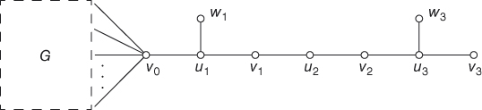
Figure 7.1 Padding for VC, with y = 101.
Example 7.12
Example 7.13
In the above examples, the padding functions are obviously length-increasing. In general, though, this property of the padding function is not necessary, as shown in the following improvement over Corollary 7.9.
Theorem 7.14
Proof
It would be interesting to know, without knowing that A or B is paddable, whether ![]() and
and ![]() are sufficient for
are sufficient for ![]() . It is an open question.
. It is an open question.
7.3 Density of NP-Complete Sets
We established, in the last section, a proof technique with which we were able to show that many natural NP-complete languages are p-isomorphic to SAT. This proof technique is, however, not strong enough to settle the Berman–Hartmanis conjecture, as we do not know whether every NP-complete set is paddable. Indeed, we observe that if all NP-complete sets are p-isomorphic to each other, then ![]() . To see this, we observe that a finite set cannot be p-isomorphic to an infinite set. Thus, if the Berman–Hartmanis conjecture is true, then every nonempty finite set is in P but is not NP-complete and, hence, is a witness for
. To see this, we observe that a finite set cannot be p-isomorphic to an infinite set. Thus, if the Berman–Hartmanis conjecture is true, then every nonempty finite set is in P but is not NP-complete and, hence, is a witness for ![]() . From this simple observation, we see that it is unlikely that we can prove the Berman–Hartmanis conjecture without a major breakthrough. Nevertheless, one might still gain some insight into the structure of the NP-complete problems through the study of this conjecture. In this section, we investigate the density of NP-complete problems and provide more support for the conjecture.
. From this simple observation, we see that it is unlikely that we can prove the Berman–Hartmanis conjecture without a major breakthrough. Nevertheless, one might still gain some insight into the structure of the NP-complete problems through the study of this conjecture. In this section, we investigate the density of NP-complete problems and provide more support for the conjecture.
The density (or the census function) of a language A is a function ![]() defined by
defined by ![]() , that is,
, that is, ![]() . Recall that a language A is sparse if there exists a polynomial q such that for every
. Recall that a language A is sparse if there exists a polynomial q such that for every ![]() ,
, ![]() .
.
Theorem 7.15
Proof
Corollary 7.16
Proof
In the following, we will show that the conclusions of Corollary 7.16 hold true even without the assumption of the Berman–Hartmanis conjecture. Thus, this provides a side evidence for the conjecture.
The proofs of these results use the self-reducibility property of NP-complete sets. We first investigate the notion of self-reducibility. This notion can be explained easily by the example of SAT.
Example 7.17
In general, different types of self-reducibility can be defined from different types of reducibility. For instance, the above self-reducibility of the problem SAT is a special case of d-self-reducibility. In order to define them, we first define a class of polynomial-time truth-table reducibilities (cf. Exercise 2.14). Recall that for a set B, χB is its characteristic function: ![]() if
if ![]() and
and ![]() if
if ![]() .
.
Definition 7.18
For instance, for ![]() , let
, let
Then, ![]() via the following TMs M1 and M2:
via the following TMs M1 and M2: ![]() for any
for any ![]() and any
and any ![]() , and M2 accepts
, and M2 accepts ![]() , where
, where ![]() , if and only if the rightmost symbol of x is equal to τ.
, if and only if the rightmost symbol of x is equal to τ.
It is easy to see that ![]() implies
implies ![]() and
and ![]() implies
implies ![]() for all k ≥ 1.
for all k ≥ 1.
Now, for each type of the reducibilities ![]() ,
, ![]() , and
, and ![]() , we define a corresponding notion of self-reducibility. We say a partial ordering
, we define a corresponding notion of self-reducibility. We say a partial ordering ![]() on
on ![]() is polynomially related if there exists a polynomial p such that (i) the question of whether
is polynomially related if there exists a polynomial p such that (i) the question of whether ![]() can be decided in
can be decided in ![]() moves; (ii) if
moves; (ii) if ![]() , then
, then ![]() ; and (iii) the length of any
; and (iii) the length of any ![]() -decreasing chain is shorter than p(n), where n is the length of its maximal element.
-decreasing chain is shorter than p(n), where n is the length of its maximal element.
Definition 7.19
Example 7.17 showed that SAT is d-self-reducible, with the natural ordering ![]() : if G is a formula obtained from F by substituting constants 0 or 1 for some variables in F, then
: if G is a formula obtained from F by substituting constants 0 or 1 for some variables in F, then ![]() . Let us look at another example.
. Let us look at another example.
Example 7.20
As shown in the above examples, each instance of a self-reducible set has a self-reducing tree. The structure of these self-reducing trees provides an upper bound for the complexity of the set.
Proposition 7.21
Proof
Are the converses of the above proposition true? That is, are all sets in PSPACE tt-self-reducible and are all sets in NP d-self-reducible? These are interesting open questions. In the following, we are going to show that a tt-self-reducible set cannot be sparse unless it is in P (Theorem 7.22(b)). Therefore, unless all sets in ![]() are nonsparse, the answer to the first question is no. By a simple padding argument, it can be proved that if
are nonsparse, the answer to the first question is no. By a simple padding argument, it can be proved that if ![]() , then there exists a tally set in
, then there exists a tally set in ![]() (cf. Exercise 1.30). Thus, if
(cf. Exercise 1.30). Thus, if ![]() , then the answer to the first question is no.
, then the answer to the first question is no.
Similarly, Theorem 7.22(a) shows that a c-self-reducible set cannot be sparse. So, it follows that the answer to the second question is also no unless there is no co-sparse set in ![]() . Or, equivalently, if
. Or, equivalently, if ![]() , then the answer to the second question is also no.
, then the answer to the second question is also no.
Are all PSPACE-complete sets tt-self-reducible, and are allNP-complete sets d-self-reducible? We do not know the precise answer. Note that it is easy to show that d-self-reducibility is preserved by polynomial-time isomorphisms (see Exercise 7.6). Thus, if the Berman–Hartmanis conjecture and its PSPACE version are true, then the answers to both of the above questions are yes. On the other hand, this property is, like paddability, easy to verify for natural problems but appears more difficult to prove for all complete problems by a general method.
We now prove our first main result of this section: tt- and c-self-reducible sets cannot be sparse, unless they are in P. It follows that PSPACE- and coNP-complete sets are not sparse unless PSPACE or NP collapses to P, respectively.