
Chapter 5
Reservoir Characterization of Unconventional Gas Formations
Abstract
Unconventional gas reservoirs have shifted the focus to special considerations of fundamentals of reservoir engineering. All reservoir characterization tools as well processing techniques are uniquely designed for conventional reservoirs. Using the tools and techniques to unconventional reservoirs has the risk of conclusions that are irrelevant and random at best. The main mechanism of fluid flow in unconventional reservoirs is through fractures, natural or induced, whereas existing techniques do not integrate this aspect to reservoir characterization. This chapter presents a new reservoir characterization technique that is suitable for unconventional reservoirs.
Keywords
knowledge model; fracture analysis; dual porosity; NMR; instability number; Representative elemental volume (REV)5.1. Summary
Unconventional gas reservoirs have shifted the focus to special considerations of fundamentals of reservoir engineering. All reservoir characterization tools as well processing techniques are uniquely designed for conventional reservoirs. Using the tools and techniques to unconventional reservoirs has the risk of conclusions that are irrelevant and random at best. The main mechanism of fluid flow in unconventional reservoirs is through fractures, natural or induced, whereas existing techniques do not integrate this aspect to reservoir characterization. This chapter presents a new reservoir characterization technique that is suitable for unconventional reservoirs.
5.2. Introduction
All consolidated petroleum reservoirs contain natural fractures or fissures. Natural fractures result from the interaction of earth stresses; whereas artificial fractures result from drilling activities, increase in pore pressure in injection operations, reservoir cooling during water flooding, redistribution of earth stresses in the field as a result of injection and production practices, etc.
Maximizing economic recovery from naturally fractured reservoirs is a complex process. It requires a thorough understanding of matrix flow characteristics, fracture network connectivity, and fracture–matrix interaction. It involves knowing the geological history. Therefore, key to successful reservoir characterization is in connecting with geologists that can construct an overall picture of the reservoir history. Construction of this history is pivotal. This construction must be scientific, following objective systematic abstraction. This is shown in Figure 5.1. The abstraction process has to be bottom up. It involves collecting data in its raw form. These data have to be collected in proper time sequence and at each step, verified from multiple sources. Medieval scholar, Alkindus famously said, “Multi-source information is a treasure.” Reservoir description should rely on information from many sources. For petroleum reservoir applications, abstraction starts with collection of geological data. In the first phase of abstraction, depiction of the subsurface strata is made. In order to create this picture, geologists must collect data from any available source, such as outcrop, regional subsurface maps. Based on this geological map, the decision to conduct geophysical survey is made. During the geophysical survey, decisions to implement a certain grid, type of survey, etc., have to be made. The process of geophysical survey offers an example of how multisource data must be integrated. During this process, geological data are used as a baseline, whereas geophysical data are later used to refine geological data. At the end, decision to drill is made only after several cycles of abstraction and refinement.

Figure 5.1 The knowledge model: The abstraction process must be bottom up.
Reservoir description should rely on information from many sources including static data (well logs, cores, petrophysics, geology, and seismic) and ultimately on dynamic data (formation evaluation well tests, long-term pressure transient tests, tracer tests, and longer term reservoir performance).
This process begins even before a geological survey begins. For instance, economic policies dictate to what extent exploration should be performed. During exploration, geologists become involved and need to be made integral part of the policy making. In order to refine geological findings, geophysical measurements are made and geophysical analysts are brought into the equation. Only after repeated abstraction and refinement, one decides to drill the first well. At this point, drilling engineers, reservoir engineers, and petroleum geologists become involved. Data collected during drilling already form integral basis for further abstraction and refinement of data. After a drilling operation is complete, coring, logging, and drill stem test (DST) are performed in order to refine static data and abstract dynamic data.
The idea behind reservoir characterization is to know the past. That means, knowing the following:
• Origin of fluid
• Origin of the reservoir
• Origin of the fractures
• Process of erosion, transport, and deposition
• Process of faulting, fracturing
• Process of secondary activities (leaching, cementation, etc.)
The next task in reservoir characterization is to know the present. It involves collection of mud data, drill cutting, oil and gas “shows,” pressure data, temperature data, and core data. These dynamic data are then assembled with static data in order to refine data on the following.
• Stratigraphy
• Lithology
• Fracture density
• Fracture orientation
• Nature of fractures
• Shale breaks
• “Sweet spots”
Initial static data collected during exploration process are the most valuable because it serves as the foundation. As soon as the first well is drilled, data must be collected even during the drilling process. Data on mud loss, rate of penetration (ROP), cuttings, azimuth, and others offer valuable insight for refining the subsurface picture.
The next set of data are generated during coring. These data include both cores and fluid sample. Even though seldom practiced, fluid data and core data should be treated like geological and geophysical data that are used for abstraction and refinement in a cyclical mode.
The core data offer the first set of direct evidence of fractures. These data should be compared with the fault network predicted in the geological map that was refined after the geological survey. Cores also give one an opportunity to determine fracture frequency, nature of fractures (e.g., plugged or open), and thus, lead toward developing the rose diagram. The development of the rose diagram is of utmost importance because that would dictate the direction of flow.
The DST data are the first set of dynamic data available. Any discrepancy between core and DST permeability would indicate the existence of fractures. As a well is put on production, it continues to generate dynamic data that are invaluable for the abstraction and refinement process, outlined above.
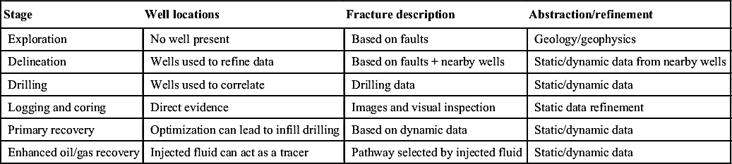
During the production cycle of a petroleum reservoir, it continues to provide one with valuable data on fracture characterization. Table 5.1 shows how fracture characteristics can be predicted with the data available at each stage of petroleum operations.
5.3. Origin of Fractures
Characterization of fracture networks is a pragmatic process that relies heavily on experience and empiricism and very little (to date) on systematic approaches. Reservoir description should rely on information from many sources including static data (well logs, cores, petrophysics, geology, and seismic) and ultimately on dynamic data (formation evaluation well tests, long-term pressure transient tests, tracer tests, and longer term reservoir performance).
Unconventional gas reservoirs are unique in many respects. Even though they are lumped into one category having a permeability value less than 0.1 mD, each type is unique and in need of independent characterization tool. It is so because none of the characterization tool is universally applicable based on only one property, i.e., permeability. For instance, sandstone has conventional oil and gas even though the formation itself is unconventional. The main difficulty in sandstone is that fracture network is not well developed due to lack of proper method that includes fracture properties. For instance, not a single core analysis technique can shed light on fracture properties of a rock. In fact, the presence of fractures or even fissures disqualifies core analysis plugs from being considered for further analysis. While several logging tools have emerged that can identify fractures, there is no systematic process to integrate that information into a reservoir characterization tool.
Shale gas plays differ from conventional gas plays in that the shale formations are both the source rocks and the reservoir rocks. There is no migration of gas as the very low permeability of the rock causes the rock to trap the gas and it forms its own seal. The gas can be held in natural fractures or pore space or can be absorbed onto the organic material. Apart from the permeability, total organic content (TOC) and thermal maturity are the key properties of gas potential shale. Generally, it can be stated that the higher the TOC, the better the potential for hydrocarbon generation. In addition to these characteristics, thickness, gas in place, mineralogy, brittleness, pore space, and the depth of the shale gas formation are other characteristics that need to be considered for a shale gas reservoir to become a successful shale gas play. The organic content in these shales, which is measured by their TOC ratings, influences the compressional and shear velocities as well as the density and anisotropy in these formations. Consequently, it should be possible to detect changes in TOC from the surface seismic response.
Table 5.1
Various Stages of Fracture Data Collection
| Stage | Well locations | Fracture description | Abstraction/refinement |
| Exploration | No well present | Based on faults | Geology/geophysics |
| Delineation | Wells used to refine data | Based on faults + nearby wells | Static/dynamic data from nearby wells |
| Drilling | Wells used to correlate | Drilling data | Static/dynamic data |
| Logging and coring | Direct evidence | Images and visual inspection | Static data refinement |
| Primary recovery | Optimization can lead to infill drilling | Based on dynamic data | Static/dynamic data |
| Enhanced oil/gas recovery | Injected fluid can act as a tracer | Pathway selected by injected fluid | Static/dynamic data |
Coalbed methane (CBM) is a gas formed as a part of the geological process of coal generation and is contained in varying quantities within all coal. CBM is exceptionally pure compared to conventional natural gas, containing only very small proportions of “wet” compounds (e.g., heavier hydrocarbons such as ethane and butane) and other gases (e.g., hydrogen sulfide and carbon dioxide). Coalbed gas is over 90% methane and is suitable for introduction into a commercial pipeline with little or no treatment.
From the earliest days of coal mining, the flammable and explosive gas in coalbeds has been one of mining's paramount safety problems. Over the centuries, miners have developed several methods to extract the CBM from coal and mine workings. CBM well production began in 1971 and was originally intended as a safety measure in underground coalmines to reduce the explosion hazard posed by methane.
The primary (or natural) permeability of coal is very low, typically ranging from 0.1 to 30 mD. Because coal is a very weak (low-modulus) material and cannot take much stress without fracturing, it is almost always highly fractured and cleated. The resulting network of fractures commonly gives coalbeds a high-secondary permeability (despite coal's typically low-primary permeability). Groundwater, hydraulic fracturing fluids, and methane gas can more easily flow through the network of fractures. Because hydraulic fracturing generally enlarges preexisting fractures and rarely creates new fractures, this network of natural fractures is very important for the extraction of methane from the coal. This is in stark contrast to what happens in sandstone formations.
Yet, gas hydrates, another unconventional natural gas source, make up completely different set of properties. Gas hydrates can be found on the seabed, in ocean sediments, in deep lake sediments, as well as in the permafrost regions. The amount of methane potentially trapped in natural methane hydrate deposits may be significant, which makes them of major interest as a potential energy resource. This methane is also of high quality.
In this chapter, a reservoir characterization technique is proposed that is applicable to all categories with the exception of gas hydrate.
5.4. Seismic Fracture Characterization
As discussed in Chapter 4, any rock deformation is the result of tectonic events that are a unique function of time. With time, events such as magma movement, faulting, earthquake, and fracturing occur in a cyclical form. It is recognized that the state of stress changes with time, affecting rock deformation directly. The stress–strain relationship is different in different zones, depending on the formation, its contents, and temperatures. Two zones are identified broadly: the shallower zone (Zone 1) where any stress translates into active reaction and changes in strain, and the deeper zone (Zone 2) that is more resilient and the strain deformation is narrow. Figure 5.2 shows a schematic of this relationship.
In Zone 1, deformation causes brittle failure and rock strength is limited by frictional strength of preexisting faults or fractures, whereas in Zone 2, the prevalent temperature makes it more resilient and faults and fractures can endure greater stress. In this zone, the temperature helps make the flow more ductile with rock strength declining exponentially with increasing temperature. Few studies have investigated the deformation of rock as a function of stress and temperature. However, it is important to understand the nature of deformation as a function of these variables in order to properly characterize fractures in a reservoir.
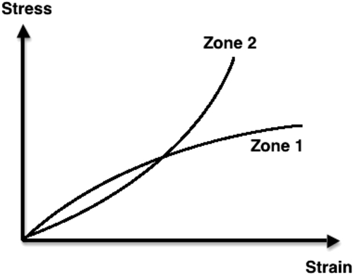
Figure 5.2 Schematic of the two zones on the earth's crustal region.
Natural fractures develop at lower temperatures with minimal stress. This is how all outcrops of consolidated rocks exhibit natural fracture networks. The existence of fracture eventually leads to the development of a fault when lateral displacement is large enough to invoke such movement across more than one sedimentary bed. This onset of fracture immediately follows the development of fissures with orientation orthogonal to the direction of fault. Depending on the nature of stress, fissures develop into fractures. These fractures become the main vehicle for hydrocarbon transport. The same fractures can onset thermal convection of water. Such flow has tremendous implication on eventual hydrocarbon generation and transport.
Two phenomena add to the complexity of fracture flow: the occurrence of shale breaks and the secondary cementation of fractures. Shale breaks decrease overall vertical permeability whereas cementation reduces overall permeability of the reservoir. For the latter, fracture orientation becomes the most important feature of fluid flow. Shale breaks, on the other hand, serves as a barrier to vertical flow and has the capacity to become a storage site for the so-called shale gas and oil. While most of the shale gas and oil reservoirs are believed to contain source rock, the shale breaks as well as caprocks also contain significant amount of gas, albeit being trapped within very low-permeability shales.
Because deeper fractures are mainly oriented normal to the direction of minimum in situ compressive stress, the presence of seismic anisotropy can signal certain pattern of fractures. While this requires true understanding of the relationships between the response of seismic anisotropy and fracture properties, the existence of seismic anisotropy offers one with the baseline for fracture characterization.
Several theoretical studies of fracture-induced anisotropy have been reported in the literature (O'Connel, R., and Budiansky, B., 1976; Budiansky, B., and O'Connel, R., 1976; Hoenig, 1979; Hudson, 1980, 1981, 1986; Crampin et al., 1986; Hudson, et al., 1996). How the presence of the fracture sets affects the elastic modulus of fractured rocks has been discussed in the literature (Schoenberg and Sayers, 1995; Thomsen, 1995; Liu et al., 1996). Based on the simplifying assumption of linear and elastic behavior, it is the background elastic modulus and fracture parameters (fracture density, aspect ratio, and saturating fluid) that determine the behavior of seismic waves, which propagate through, and are reflected from, the reservoirs.
Fracture models are based on major physical features such as the azimuthal P- and S-wave velocity variations with fracture parameters. The azimuthal variations in P-wave velocity and reflectivity in homogeneously fractured reservoirs as a function of anisotropic parameters have been described by many researchers (Tsvankin, 1996; Ruger, 1998; Al-Dajani and Tsvankin, 1998). These anisotropic parameters are related to fracture parameters through the elastic stiffness tensors. In principle, azimuthal amplitude versus offset (AVO) responses can be used to detect fractures. Successful use of azimuthal variation of P-wave AVO signatures to determine the principal fracture orientation and density have been reported in the literature (Lynn et al., 1995, 1996; Perez and Gibson, 1996).
In principle, the distribution of fractures in reservoir zones can be treated as homogeneous. In practice, the number and variability of small-scale fractures are so large that recovering significant information from P-wave seismic data requires the distribution characteristics to be averaged over the reservoir zone, which leads to a statistical representation. This is equivalent to the notion of assigning pseudo-homogeneity. Heterogeneity due to spatial variations of fracture density could result in spatial variations of velocity anisotropy. It is important to identify the coherent features in reflected seismic data. These features are often used as major seismic characteristics in exploration geophysics. The small incoherent arrivals that occur between the major reflections also contain information about the media. They are currently treated as “noise,” but contain valuable information that can alter the reservoir description if filtered correctly. Currently used techniques are not capable of analyzing these signals with scientific accuracy (Charrette, 1991). The 3D finite-difference modeling technique is effective in studying the azimuthal AVO response and scattering characteristics in heterogeneously fractured media. However, they allow no room for including “noises.” Although grid memory requirements make computations very expensive and grid dispersion effects limit finite-difference models to small regions, this approach has been successfully used to model energy diffracted at highly irregular interfaces (Lavender and Hill, 1985; Dougherty and Stephen, 1987), to study fluid-filled bore-hole wave propagation problems in anisotropic formations (Cheng et al., 1995), and to study the scattering in isotropic media (Frankel and Clayton, 1986; Coates and Charrette, 1993; Zhu, 1997). Additionally, unlike boundary integral techniques, lateral velocity variations can be easily incorporated (Stephen, 1984, 1988).
Azimuthal AVO variations have been used in fracture detection and density estimation (Perez, 1997; Ramos and Davis, 1997). However, the sensitivity of reflected P-waves to the discontinuity of elastic properties at a reflected boundary and to the spatial resolution makes it difficult to interpret this attribute unambiguously. The motivation of this thesis is to explore the efficiency, benefits, and limitations of using P-waves to characterize fractured reservoirs, theoretically and practically. Shen (1998) studied the possibility of using P-waves to investigate properties of fractured reservoirs and the diagnostic ability of the P-wave seismic data in fracture detection. This study also considered rheological behavior of rocks at a crustal scale, based on observation and modeling of continental deformation, in particular, deformation of the Tibetan plateau. The Tibetan plateau is an ideal location that features continental topography, resulting from the N–S convergence between the Indian and Eurasian plates.
5.4.1. Effects of Fractures on Normal Moveout (NMO) Velocities and P-Wave Azimuthal AVO Response
Shen (1998) investigated the effects of fracture parameters on anisotropic parameter properties and P-wave NMO velocities, based on developed effective medium models and crack models. Anisotropic parameters of the pseudo-transversely isotropic medium model, S(v) and E(v), have different characteristics in gas- and water-saturated, fractured sandstones. When fractures are gas-saturated, δ(v) and ε(v) vary with the fracture density alone. In water-saturated, fractured sandstones, both δ(v) and ε(v) depend on fracture density and crack aspect ratio. δ(v) is related to the Vp/Vs of background rocks and ε(v) is a function of the Vp of background rocks. Studies show that the shear wave splitting parameter, γ(v), is most sensitive to crack density and insensitive to saturated fluid content and crack aspect ratio. Properties of P-wave NMO velocities in a horizontally layered medium are the function of δ(v). The effects of fracture parameters on P-wave NMO velocities are comparable with the influences of δ(v).
P-wave azimuthal AVO variations are not necessarily correlated with the magnitude of fracture density. Shen (1998) showed that the elastic properties of background rocks have an important effect on P-wave azimuthal AVO responses. Results from 3D finite-difference modeling show that azimuthal AVO variations at the top of gas-saturated, fractured reservoirs, which contain the same fracture density, are significant in the reservoir model with small Poisson's ratio contrast. Analytical solutions indicate that azimuthal AVO variations are detectable when fracture-induced reflection coefficients can generate a noticeable perturbation in the overall reflection coefficients. Varying fracture density and saturated fluid content can lead to variations in AVO gradients in off fracture strike directions. Shen's numerical results also show that AVO gradients may be significantly distorted in the presence of overburden anisotropy caused by vertical transverse isotropy media, which suggests that the inversion of fracture parameters based on an individual AVO curve would be biased without correcting this influence. He recommended that azimuthal AVO variations could be effective for detecting fractures; model analysis studies and combination of P-wave NMO velocities are more beneficial than using reflection amplitude data alone.
5.4.2. Effects of fracture Parameters on Properties of Anisotropic Parameters and P-Wave NMO velocities
In exploration geophysics, NMO describes the effect that the distance between a seismic source and a receiver (the offset) has on the arrival time of a reflection in the form of an increase of time with offset. The relationship between arrival time and offset is hyperbolic, typically described by a wave equation. This relationship is the principal criterion that a geophysicist uses to decide whether an event is a reflection or not. The NMO depends on complex combination of factors including the velocity above the reflector, offset, dip of the reflector, and the source receiver azimuth in relation to the dip of the reflector. Of concern is the role of fractures; to understand the effect of fracture parameters on NMO velocities, one needs to understand effects of fracture parameters on anisotropic parameter properties.
Table 5.2
Elastic Parameters Used by Shen (1998)
| Sandstone no. | Vp (m/s) | Vs (m/s) | ρ (g/cm3) | Vp/Vs | References |
| No. 1 | 3368 | 1829 | 2.50 | 1.84 | Thomsen (1986) |
| No. 2 | 4405 | 2542 | 2.51 | 1.73 | Thomsen (1986) |
| No. 3 | 4539 | 2706 | 2.48 | 1.68 | Thomsen (1986) |
| No. 4 | 4476 | 2814 | 2.50 | 1.59 | Thomsen (1986) |
| No. 5 | 4860 | 3210 | 2.32 | 1.51 | Teng and Mavko (1996) |
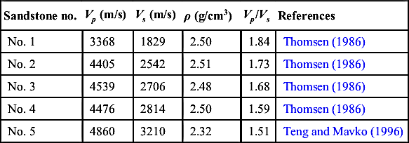
Table 5.3
Elastic Parameters and Fracture Parameters of Model 1 and Model 2
| Model | Vp (m/s) | Vs (m/s) | ρ (g/cm3) | Fracture density(%) and aspect ratio | Poisson's ratio | Type of rocks |
| Model 1 | 4358 | 3048 | 2.81 | 0.021 | Mesaverde shale | |
| 3368 | 1829 | 2.50 | 10 0.01 | 0.291 | Taylor sandstone | |
| Model 2 | 4561 | 2988 | 2.67 | 0.124 | Shale | |
| 4860 | 3210 | 2.32 | 10 0.01 | 0.113 | Sandstone |
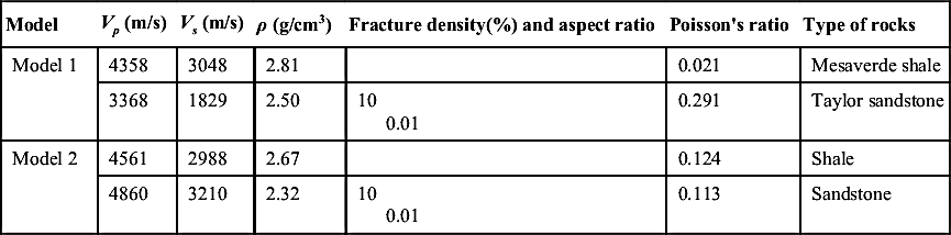
Shen (1998) studied various elastic parameters of five sandstones, whose characteristics are summarized in Tables 5.2 and 5.3. He studied for two aspect ratios, i.e., 0.01 and 0.05. Figure 5.3 shows δ(v) as a function of fracture density for a gas-saturated sandstone with fracture aspect ratio of 0.01. Results are shown for an aspect ratio of 0.05 (Figure 5.4). These results show that for gas-saturated sandstones, δ(v) is insensitive to aspect ratio. For the water-saturated case, however, absolute values of δ(v) increase with fracture density and crack aspect ratio. This latter case (Figures 5.5 and 5.6) also shows a range of values for different samples, as compared to gas-filled case that show little dependence on sample types. It is also noted that δ(v) is dependent on Vp/Vs of isotropic, unfractured sandstones. The smaller the Vp/Vs, the larger the absolute value of δ(v) obtained.
ε(v) shows similar characteristics to δ(v). The difference is that ε(v) is the function of the Vp of the background medium. In gas-saturated, fractured sandstones, ε(v) is sensitive to fracture density alone. In water-saturated, fractured sandstone the absolute value of ε(v) increases with both fracture density and aspect ratio. The smaller the Vp, the smaller the absolute value ε(v) obtained. ε(v) as a function of fracture density and crack aspect ratio in gas- and water-saturated, fractured sandstones is shown in Figures 5.7 through 5.9.
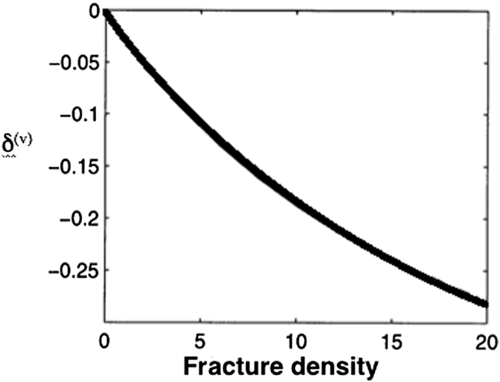
Figure 5.3 Variation in anisotropic parameter as a function of fracture density for gas-saturated sandstone and fracture aspect ratio of 0.01. Redrawn from Shen, 1998.
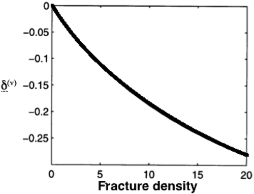
Figure 5.4 Variation in anisotropic parameter as a function of fracture density for gas-saturated sandstone and fracture aspect ratio of 0.05. Redrawn from Shen, 1998.
Parameter γ(v), is different from both δ(v) and ε(v) in that it measures the degree of shear wave splitting at vertical incidence. Figures 5.10 through 5.13 show that γ(v) has little dependence on fluid bulk modulus and crack aspect ratio and is the parameter most directly related to fracture density. Therefore, for parallel, penny-shaped cracks, the shear wave splitting parameter, γ(v), can provide direct information about fracture density with least ambiguity.
These findings show that the variations of parameters δ(v) and ε(v) are sensitive to fluid content. For gas-saturated fractures, δ(v) and ε(v) vary with the fracture density alone, making them an effective indicator of fractures. On the other hand, for water-saturated fractures, the magnitudes of δ(v) and ε(v) depend on fracture density, crack aspect ratio, and elastic properties of background rocks. Whereas the shear wave splitting parameter, γ(v), is insensitive to both fluid content and crack aspect ratio. It is the parameter most related to crack density. P-wave NMO velocity is controlled by the vertical P-wave velocity, angle between crack normal and survey line, and the parameter δ(v).
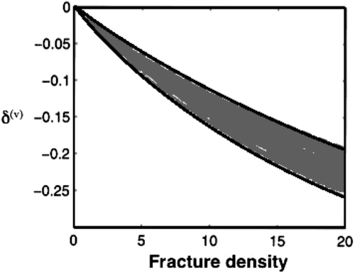
Figure 5.5 Range of variation in anisotropic parameter as a function of fracture density for water-saturated sandstone and fracture aspect ratio of 0.01. Redrawn from Shen, 1998.
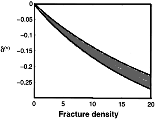
Figure 5.6 Range of variation in anisotropic parameter as a function of fracture density for water-saturated sandstone and fracture aspect ratio of 0.05. Redrawn from Shen, 1998.
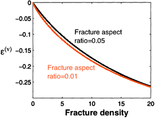
Figure 5.7 Variation in anisotropic parameter as a function of fracture density for gas-saturated sandstone and fracture aspect ratio of 0.01 and 0.05. Redrawn from Shen, 1998.
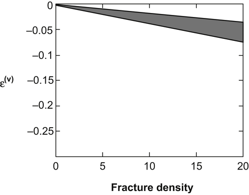
Figure 5.8 Range of variation in anisotropic parameter as a function of fracture density for water-saturated sandstone and fracture aspect ratio of 0.01. Redrawn from Shen, 1998.
5.5. Reservoir Characterization during Drilling
It is generally understood that vast unconventional gas resources are accessible only with more advanced techniques. Cost-effective drilling techniques and well completion strategies constitute the most successful technological development in the petroleum industry. At present, 90% of the new wells drilled are horizontal. These wells are likely to intersect natural fractures that are predominantly vertical in unconventional reservoirs. Drilling and completion of horizontal wells and multilaterals have been the cornerstone of successful unconventional gas recovery schemes. Drilling in this type of formations is often optimized with the so-called managed pressure drilling (MPD). MPD uses tools at the surface such as a choke to control the drilling fluid flow rate and bottomhole pressure. The various drilling operations that MPD comprised of provide economical solutions to many drilling problems such as managing gas kicks, lost circulation and other well control issues, improving ROP, minimizing formation damage, and enabling dynamic reservoir characterization from real-time mud log data (Ramalho et al., 2009). Underbalanced drilling (UBD) is a form of MPD that is particularly useful when drilling horizontal wells in tight gas formations. It also generates data that can turn it into a dynamic reservoir characterization tool.
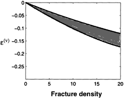
Figure 5.9 Range of variation in anisotropic parameter as a function of fracture density for water-saturated sandstone and fracture aspect ratio of 0.05. Redrawn from Shen, 1998.
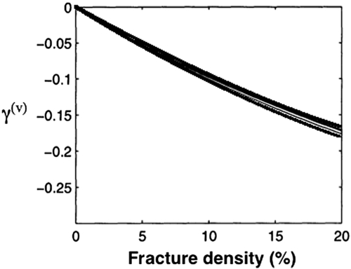
Figure 5.10 Range of variation in shear wave splitting parameter as a function of fracture density for gas-saturated sandstone and fracture aspect ratio of 0.01. Redrawn from Shen, 1998.
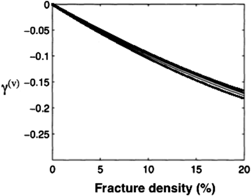
Figure 5.11 Range of variation in shear wave splitting parameter as a function of fracture density for gas-saturated sandstone and fracture aspect ratio of 0.05. Redrawn from Shen, 1998.
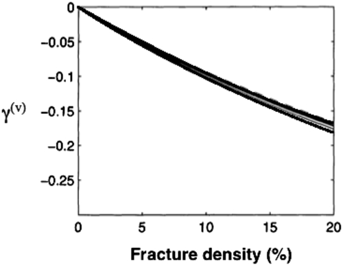
Figure 5.12 Range of variation in shear wave splitting parameter as a function of fracture density for water-saturated sandstone and fracture aspect ratio of 0.01. Redrawn from Shen, 1998.
As shown in Table 5.1, the first set of direct data is produced during drilling. As soon as drilling is commenced, the drilling log becomes available. The drilling log contains information about the progress of the well such as measured depth (MD), true vertical depth, inclination, weight on bit, ROP, and gamma ray. It also provides information about the drilling mud circulation system such as mud pit volume, pump pressure, and mud flow rate. Each of these data is valuable for description of lithology as well as fracture system of a formation.
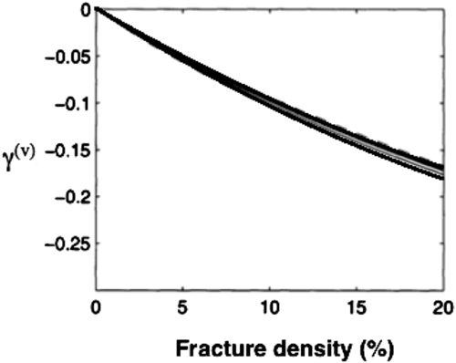
Figure 5.13 Range of variation in shear wave splitting parameter as a function of fracture density for water-saturated sandstone and fracture aspect ratio of 0.05. Redrawn from Shen, 1998.
Any drilling process also accompanies the mud log. This log is generally created by the on-site geologist as the well is drilled. Mud logs contain valuable information regarding formation geology and hydrocarbon in place. As the drill bit penetrates the formation, the rock is crushed, and these cuttings are flushed from the well and carried to the surface by the circulating drilling mud. A geologist routinely examines the cuttings and describes the lithology of the formation being penetrated. This information is recorded in the mud log on a depth basis as the well is drilled in order to create a geologic profile of the entire well. At the same time, total gas measurements are also made and recorded. Total gas measurements indicate the relative concentration of hydrocarbons (methane, ethane, propane, etc.) present in the circulating drilling mud at any given time.
During conventional drilling operations, the drilling mud density is maintained above the reservoir pore pressure for wellbore stability issues. While, during this overbalanced drilling useful data are generated that can indicate the presence of fractures and sweet spots (e.g., mud loss, fluid loss, high ROP), information regarding fluid in place is limited. In such system, produced fluids can only occur when an unexpected overpressured zone is encountered or when a transient mud pressure reduction occurs as the drill string is raised (swabbing). Ever since the advent of UBD that uses mud pressure lower than pore pressure, the possibility of extracting in situ fluid in order to characterize the reservoir has been increased drastically. During UBD, hydrocarbon production will occur consistently during drilling, whenever a sweet spot is penetrated. Such “sweet spots” can be the result of natural fractures or otherwise high-permeability zones. Produced fluid as a result of the underbalanced pressure condition is a major focus of this investigation. Recycled fluids may occur if the gas contained within the circulating mud is not entirely released at the surface. In this instance, the remaining gas will be recirculated through the system and will be detected again on the next pass. Finally, contamination will always occur due to various unavoidable causes. Reasons for contamination of the total gas readings include petroleum products intentionally added to the drilling mud, chemical reactions, and degradation of organic mud additives, and even emissions from construction equipment on-site. It is very important to understand all of these processes so that one can effectively interpret the mud log analysis.
The drilling fluid circulation system is essentially a closed-loop system in which the mud is pumped down the well through the center of the drill string, flows through the drill bit nozzle, and is then forced back up to the surface through the annular section. This process ensures that the drill bit stays cool, creates a hydrostatic pressure that is exerted against the wellbore wall for well stability issues and flushes the cuttings to the surface. At the surface, the mud is transported through a shaker table to remove the cuttings and then released into a mud pit to complete the cycle. To obtain the total gas measurements, a gas trap is installed at the mud pit that is able to capture a sample of gas from the mud. An impeller agitates the mud releasing gas into the air. A mixture of this gas–air sample is then sent to the mud logging unit for analysis. The total gas reading is a measure of the relative concentration of all hydrocarbons combined. This concentration is recorded along depth of the drill bit. A correction may be necessary to account for the mud travel time.
While “gas shows” are routinely used to delineate productive zones as well as plan completion strategies, they can also serve as a tool for formation characterization. This is particularly important for unconventional gas reservoirs.
Most unconventional reservoirs are known to contain a high density of natural fractures and production is in fact dominated by fracture flow. Typically, it is presumed that vertical natural fractures exist in situ. Therefore, to produce economically from these types of reservoirs it is most efficient to drill horizontal wellbores. The lateral sections of these wellbores are often drilled underbalanced. During UBD operations, gas is expected to flow into the wellbore consistently throughout the drilling process. The combination of low-permeability matrix, high-permeability natural fractures, and the underbalanced pressure condition leads to the result of highly complicated mud logs. However, a thorough analysis of the mud log data can reveal critical information about the natural fracture system near the wellbore.
The fundamental premise of this analysis is that for unconventional reservoirs, the bulk of the fluid flow takes place through fractures. Such premise is justified based on Darcy's law:
⇀v=−kμ∇P
![]() (5.1)
(5.1)
Here ⇀v is the velocity, k is the permeability, μ is the viscosity, and P is the pressure. Permeability has the dimension of L2, which means it is exponentially higher in any fracture than the matrix. For a system with very low permeability, fracture flow accounts for 99% of the flow, whereas in terms of volume fractures account for 1% of the volume of the void (or total porosity). This is significant, because in classic petroleum engineering, governing equations are always applied without distinction between storage site (where porosity resides) and flow domain (where permeability is conducive to flow). In unconventional reservoirs, fluid flow equations apply to the fracture network whereas storage volume applies to the matrix that has little permeability. In fact, permeability values are so low in the matrix, typical Darcy's law does not apply to this domain. It is recommended that Forchheimer equation can be used to describe gas flow. This equation is given by:
−∇P=μkv+ρβv2
![]() (5.2)
(5.2)
In the above equation, β is an additional proportionality constant that depends on rock properties. For a system with predominant fracture flow, β would depend on the fracture density and aspect ratio.
In case, fracture network is insignificant and the reservoir matrix permeability is very low, flow in such system is best described with Brinkman equation, described as:
−∂P∂x=uμk−μ∂2u∂x2.
![]() (5.3)
(5.3)
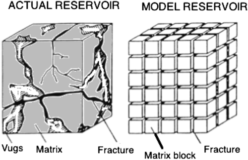
Figure 5.14 Depiction of Warren and Root model.
To date, the most commonly used model is that proposed by Warren and Root (1965). This so-called dual porosity model (Figure 5.14) assumes that two types of porosity are present in the formation, one arising from vugs and fracture system, whereas the other from matrix. For unconventional reservoirs, the matrix permeability is negligible compared to fracture permeability (hence depicted with shades). Warren and Root invoked similar assumptions even for a matrix with relatively high permeability. The approach operates on the concept that fractures have large permeability but low porosity as a fraction of the total pore volume. The matrix rock has the opposite properties: low permeability but relatively high porosity. This approach describes the observation that fluid flow will only occur through the fracture system on a global scale. Locally, fluid may flow between matrix and fractures through interporosity flow, driven by the pressure gradient between matrix and fractures.
Fracture flow is described by Snow's equation (1963), given below:
QΔP=Cw3
![]() (5.4)
(5.4)
Here w is the fracture aperture and C is a proportionality constant that depends on the flow regime that prevails in the formation. Snow's equation emerges from a simple synthesis of parallel plate flow (Poiseuille law) that assumes permeability to be b2/12, where b is the fracture width.
Fracture geometries are often idealized to simplify modeling efforts. In most cases the width is assumed to be constant, and the fracture is usually considered either a perfect rectangle or a perfect circle. In reality, fracture geometries are very complex (Figure 5.14), and many different factors could affect the behavior of fluid flow. In Figure 5.14 that was originally published by Warren and Root (1965), vugs are shown prominently. It is no surprise that they introduced the concept of dual porosity. Indeed, porosity in vugs and in matrix is comparable. For unconventional reservoirs, however, the vugs are nonexistent and most fractures have very little storage capacity, making their porosity negligible to that of the matrix. In determining sweet spots within an unconventional reservoir, the consideration of very high fracture to matrix permeability, kf/km is of importance. For application in dynamic reservoir characterization using real-time mud log data, the term “sweet spot” is used when the drill bit intersects a transverse natural fracture. Such process is equivalent to numerous passes of history match in the context of reservoir simulation.
5.5.1. Overbalanced Drilling
Overbalanced drilling approaches for fracture characterization mostly consist of methods that take advantage of mud-loss data and the rheological properties of the circulating drilling fluid. Drilling mud is usually a non-Newtonian fluid that exhibits shear-thinning behavior. Shear thinning implies that the fluid viscosity decreases with an increase in the shear rate. During drilling, the drilling mud is constantly circulated through a closed-loop system. If the circulation is stopped, the drilling mud will develop into a thick gel. The mud will remain in this state until a pressure exceeding the mud's yield stress is applied, at which point it will return to its “fluid” state. This nonideal fluid behavior has allowed engineers to develop methods to characterize fracture permeability using mud-loss data. In a dynamic setting, mud rheology can be calibrated against mud circulation loss, which is directly related to fracture in an unconventional tight gas reservoir.
During overbalanced drilling, when a sweet spot is encountered, the mud pressure is greater than the fluid pressure contained in the fracture resulting in a flood of drilling mud into the fracture. When the drill bit intersects the fracture, drilling mud will flow into the fracture. Because the matrix permeability is low, leak off into the matrix is minimal and the mud loss is entirely due to fluid flow through fractures.
This mud flow is reflected in the rheology of the returning mud, thereby, creating a correlation between surface-observed rheology and fracture density as well as fracture geometry (Figure 5.15).
Lietard et al. (1999) provide type curves describing mud-loss volume versus time that can be used to determine the hydraulic width of fractures through a curve matching approach. The type curves are based on an analysis of the local pressure drop in the fracture (Lietard et al., 1999):
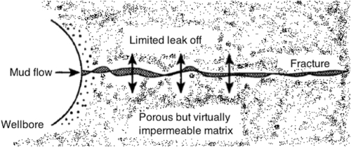
Figure 5.15 Schematic of mud flow in a tight formation with fractures. After Dyke et al., 1995.
dPdr=12μpvmw2+3τyw
![]() (5.5)
(5.5)
Where, vm is the local velocity of the mud in the fracture, μp is the plastic viscosity of the mud, w is the fracture aperture, and τy is the yield stress of the mud. This equation was improved by Huang et al. (2010) that suggested the following equation:
(ΔPOBτy)2w3+6Rw(ΔPOBτy)w2−9π(Vm)max=0
 (5.6)
(5.6)
In the above equation, Rw is the well radius and Vm is the maximum mud-loss volume. This equation is easier to use than the previously used type curve. However, it is recommended that such correlation be developed for each reservoir.
5.5.2. Underbalanced Drilling
During UBD operations, a low density drilling fluid is used in order to maintain a wellbore pressure profile that is lower than the pore pressure of the formation at all locations along the borehole. One major advantage of UBD over conventional drilling is that formation damage is reduced because a filter cake is not allowed to form near the wellbore. Wells completed with UBD have been shown to perform three to four times better than their conventional counterparts in the same formation. Among others, lost circulation is minimized with UBD. Overall, the ROP is increased significantly with UBD. Figure 5.16 shows how switching from overbalanced drilling to UBD can drastically increase ROP. This is especially true for tight gas formations or any formation with harder than normal. This phenomenon is not well understood, but it is thought that the increased ROP can be attributed to the lower confining pressure on the formation rock under UBD conditions and to the fact that cuttings are more easily flushed from the bottom of the wellbore reducing the resistance on the drill bit.
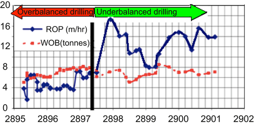
Figure 5.16 Data from a well drilled overbalanced until a certain depth and then switching to underbalanced operations. Immediately as UBD begins, the ROP greatly increases. Redrawn from Woodrow et al., 2008.
The most useful aspect of UBD is in the insight gained during UBD. The deliberate underbalanced pressure difference between the drilling fluid and the formation pressure causes an inflow of formation fluid into the wellbore along the entire drilled section. This can act as a tracer for dynamic reservoir characterization.
The most important piece of data is the rate of fluid flow from the formation into the wellbore. Very rarely are flow rates actually measured at bottomhole. In almost all cases, the formation fluid-flow rate is estimated from surface measurements of inflow and outflow of the drilling fluid. The difference between the mud injected into the wellbore and the outflow of mud from the annular section is often estimated as the formation fluid-flow rate. Methods to account for the expansion of gas due to changes in temperature and pressure must be taken into account to obtain accurate data (Aremu and Osisanya, 2008). Other data that models tend to utilize include bottomhole pressure, ROP, formation porosity, wellbore diameter, and wellbore length. Models generally provide profiles of formation permeability and pore pressure versus depth. Norbeck (2012) presented field data, showing correlation between UBD data and fractures. He extracted field data originally reported by Myal and Frohne (1992). The report investigates the effectiveness of directional drilling in a tight gas formation located in the Piceance Basin of western Colorado. The formation is known to be highly naturally fractured, and consequently the decision was made to drill a large section of the well underbalanced in order to reduce formation damage and lost circulation. As can be seen from Figure 5.17, at least 10 major gas shows were detected during drilling. These gas shows were attributed to the presence of natural fractures intersected by the wellbore. An increase in mud density not only led to suppression of the gas shows, but also prevented extraction of gas show data and their correlation with fracture distribution. This type of correlation can lead to depiction of the formation fracture network.
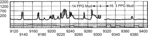
Figure 5.17 Mud log data from a portion of a well, drilled underbalanced in the Piceance Basin. The large gas peaks were attributed to natural fractures that were intersected by the wellbore. Redrawn from Myal and Frohne, 1992.
Norbeck (2012) proposed two criteria that can be combined to develop a correlation between mud log data and reservoir properties. They are:
Criterion 1: The first criterion is the use of total gas concentration measurements from mud logs. Using a gas chromatograph, the mud logging unit is able to determine the concentration of gas present in the drilling fluid at any given time. As natural fractures are intersected by the drilling bit, gas flows into the wellbore and the amount of gas is proportional to the average fracture permeability. These concentration values show up as spikes on the total gas concentration of mud log.
Criterion 2: The second criterion is based on observations of the mud pit volume. Observations of the mud pit volume at the surface also show potential as a fracture identification criterion. It is widely accepted that decreases in mud pit volume (mud losses) correspond to encounters with natural fractures while drilling overbalanced. It is logical to assume that the reverse is also true during UBD. It means that as a natural fracture is encountered with the drill bit, the formation fluid influx will cause a displacement of drilling fluid in the mud pit. This response is observable at the surface.
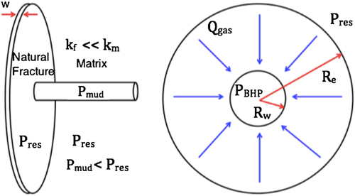
Figure 5.18 Schematic of the model used by Norbeck (2012).
Both criteria are related to open fractures that contribute to flow directly. Furthermore, fractures are uniquely correlated if the formation is tight with negligible permeability. In order to estimate natural fracture permeability, several assumptions have to be made:
1. All natural fractures that have been intersected by the wellbore are transverse to the wellbore and have circular geometry with finite extent (as depicted in Figure 5.18).
2. Natural fractures have constant aperture. At least, it must be assumed that an equivalent aperture is a reasonable and practical approximation. Tortuosity or other “eccentricity” factors can be introduced; however, simple geometry is a reasonable assumption.
3. Gas contained within natural fractures is composed 100% of methane. Methane density and viscosity remain constant while flowing through fractures. This approximation avoids the analysis of compositional effect on gas chromatography.
4. Fluid flow through fractures follows the cubic law relationship. This is typical of all existing fracture flow models. The cubic law relationship assumes steady state, laminar flow between two parallel plates. The cubic law can be derived from a force balance between the forces due to the pressure gradient and the shear resistance on the boundaries, as opposed to the diffusivity equation, which is derived using the principles of conservation of mass. As such, no compressibility term is present in the cubic law relationship. However, the high compressibility of gas will most likely have significant effects on the flow rate through the fracture. Nonetheless, it is assumed that at the high pressure conditions present in the reservoir, compressibility effects will be negligible over the relatively low magnitude pressure drop between reservoir and bottomhole pressures.
5. Matrix permeability is much lower than fracture permeability. For most unconventional reservoirs, this is a reasonable approximation.
6. No charging of the fractures occurs during the time spans considered. Considering low permeability of the matrix, this is a reasonable assumption.
7. The gas influx volume is equal to the mud pit volume increase. For most shallow reservoirs, this is a reasonable approximation. Because no direct measurements of gas flow rate at bottomhole are recorded on today's drilling rigs, it is assumed that the observed mud pit volume increase is equal to the volume of gas that entered the wellbore from the fracture. However, compressibility effects could be significant and add to the uncertainty of this analysis. Also, it is well known that methane is highly soluble in oil-based drilling mud, and it is has been reported that observations of mud pit volume increase as a response to a gas kick will be reduced because of solubility effects.
The following estimates can be obtained from the drilling and mud log data:
• Gas flow rate
• Pressure drop (underbalance)
• Methane viscosity
• Wellbore radius
If an assumption about the radial extent of the fracture can be made, then fracture aperture can be determined as follows:
w=(QCΔP)1/3
 (5.7)
(5.7)
Then, fracture permeability can be estimated by the following equation that is derived from Poiseuille law, as applied in parallel plate flow.
k=w2/12
![]() (5.8)
(5.8)
Norbeck (2012) demonstrated through study of six wells that this technique is both practical and accurate. Data from six wells that were drilled underbalanced were collected. Conductive natural fracture zones are determined for each well, thereby estimating fracture permeabilities. The wells were from two tight gas shale formations, one located in the United States and the other in Canada. The lateral sections of these horizontal wells range from 3000 to 6000 ft. The lateral sections of all wells were drilled using oil-based mud.
In order to verify accuracy of the analysis, a special technique had to be applied because no borehole image logs were available. The main validation technique used in that study took advantage of a commonly used horizontal drilling technique in which wells are drilled in parallel. Six wells selected for the study constituted three sets of parallel wells drilled to similar elevations. The spacing of these wells was between 500 and 800 ft. The parallel well sets should penetrate similar natural fracture systems. The results of the natural fracture identification analysis for each parallel well set are compared to determine if any patterns exist that may be indicative of the orientation of natural fracture planes.
Table 5.4
Length of Lateral Sections, Average True Vertical Depth (TVD) of Lateral Sections, and Average Reservoir Pore Pressures for Corresponding TVD for Wells A-1 and A-2
| Well name | Length of lateral (ft) | Average TVD of lateral (ft) | Average reservoir pressure (psi) |
| A-1 | 4280 | 12,381.8 | 11,550 |
| A-2 | 3131 | 12,389.8 | 11,575 |
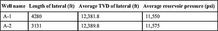
From Corbeck, 2010.
In the first field case study, first two wells (Well A-1 and Well A-2) were chosen from the same field. The horizontal spacing between these two wells is roughly 800 ft. Well A-1 runs in S–N orientation and Well A-2 runs in the opposite direction. Well A-1 was drilled toe down and Well A-2 was drilled toe up. The geometric properties and the average reservoir pressure for each well, obtained from diagnostic fracture injection testing, are listed in Table 5.4. The targeted pay zone is roughly 175-ft thick.
The analysis of Well A-1 indicates that 10 conductive natural fractures were intersected during the drilling process (see Table 5.5). Two of these natural fractures are within very close proximity to each other and are considered a single conductive natural fracture zone. In total, nine natural fracture zones are present along the lateral of this well. As can be seen in Figure 5.19, the stretch of lateral between 14,000 and 15,500 ft MD contains no conductive natural fracture zones. This is a primary example of the insight that can be gained from this type of analysis. This zone can be selected for creating sweet spots through hydraulic fracturing. The fracture apertures range from 13 to 53 μm. The cross-plot indicates a general positive correlation between mud pit volume peak and gas peak for these conductive natural fracture zones (see Figure 5.20).
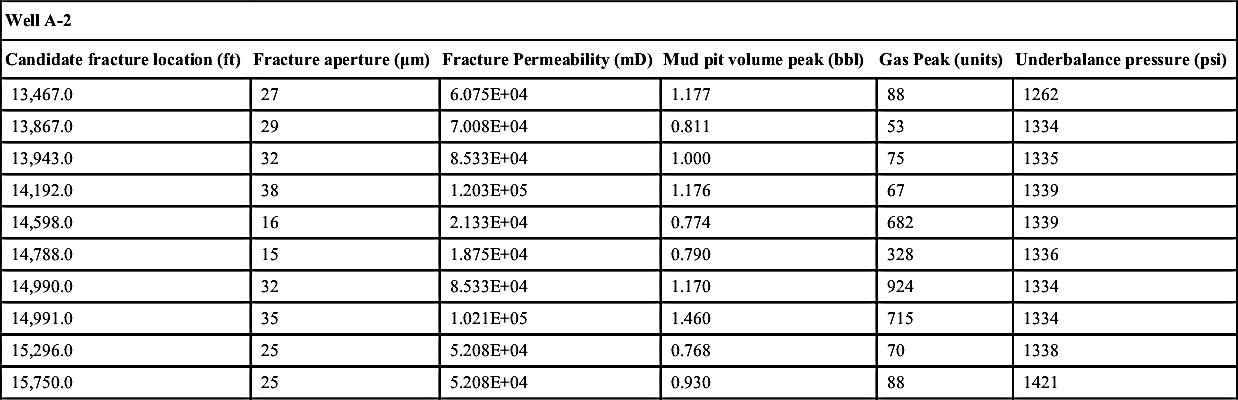
Similarly, a total of nine conductive natural fracture zones were identified for Well A-2. The relevant results are listed in Table 5.6. The zones are relatively evenly spaced along the lateral (see Figure 5.21). The fracture apertures are generally smaller than for Well A-1, ranging from 15 to 38 μm. These estimates could be largely due to the higher level of underbalance maintained while drilling Well A-2. Additionally, the observed rise in mud pit volume due to the presence of these fractures is relatively low. The cross-plot does not show a strong trend for the relationship between mud pit volume peak and gas peak for these fractures, however, it is a positive correlation (see Figure 5.22).
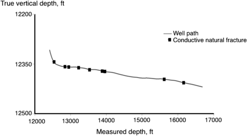
Figure 5.19 Locations of conductive natural fractures along the lateral of Well A-1. Redrawn from Corbeck, 2010.
Table 5.5
Results of Fracture Identification in Well A-1
| Well A-1 | |||||
| Candidate fracture location (ft) | Fracture aperture (μm) | Fracture permeability (mD) | Mud pit volume peak (bbl) | Gas peak (units) | Underbalance pressure(psi) |
| 12,533.0 | 30 | 7.500E+04 | 4.000 | 988 | 1093 |
| 12,826.0 | 35 | 1.021E+05 | 3.000 | 171 | 1081 |
| 12,835.0 | 53 | 2.341E+05 | 3.200 | 156 | 1081 |
| 12,950.0 | 44 | 1.613E+05 | 1.600 | 286 | 1080 |
| 13,235.0 | 42 | 1.470E+05 | 1.700 | 182 | 1143 |
| 13,529.0 | 37 | 1.141E+05 | 1.700 | 69 | 1138 |
| 13,884.0 | 36 | 1.080E+05 | 1.600 | 74 | 1135 |
| 13,960.0 | 42 | 1.470E+05 | 2.300 | 150 | 1133 |
| 15,613.0 | 35 | 1.021E+05 | 1.900 | 103 | 1178 |
| 16,156.0 | 13 | 1.408E+04 | 1.600 | 644 | 1234 |
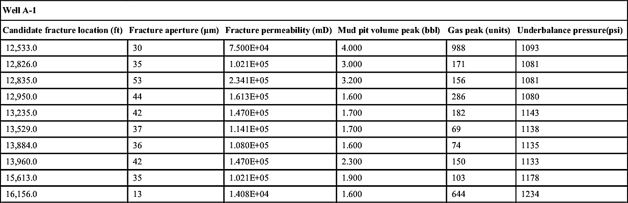
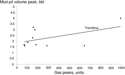
Figure 5.20 Cross-plot of mud pit volume peak versus gas peak corresponding to each conductive natural fracture location identified for Well A-1. Redrawn from Corbeck, 2010.
Table 5.6
Results of Fracture Identification in Well A-2
| Well A-2 | |||||
| Candidate fracture location (ft) | Fracture aperture (μm) | Fracture Permeability (mD) | Mud pit volume peak (bbl) | Gas Peak (units) | Underbalance pressure (psi) |
| 13,467.0 | 27 | 6.075E+04 | 1.177 | 88 | 1262 |
| 13,867.0 | 29 | 7.008E+04 | 0.811 | 53 | 1334 |
| 13,943.0 | 32 | 8.533E+04 | 1.000 | 75 | 1335 |
| 14,192.0 | 38 | 1.203E+05 | 1.176 | 67 | 1339 |
| 14,598.0 | 16 | 2.133E+04 | 0.774 | 682 | 1339 |
| 14,788.0 | 15 | 1.875E+04 | 0.790 | 328 | 1336 |
| 14,990.0 | 32 | 8.533E+04 | 1.170 | 924 | 1334 |
| 14,991.0 | 35 | 1.021E+05 | 1.460 | 715 | 1334 |
| 15,296.0 | 25 | 5.208E+04 | 0.768 | 70 | 1338 |
| 15,750.0 | 25 | 5.208E+04 | 0.930 | 88 | 1421 |
Similar results were obtained for other fields as well. On average, the computational tool identifies between nine and ten conductive natural fracture zones for each well. For each conductive natural fracture zone, the fracture aperture and fracture permeability was estimated. The estimated fracture apertures all lie within the expected range of values (i.e., 10–1000 μm). Overall, although the estimates of fracture aperture may not be entirely accurate, they should be considered as a lower bound for the true fracture apertures.
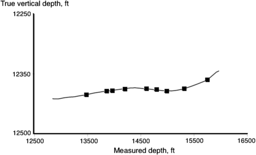
Figure 5.21 Locations of conductive natural fractures along the lateral of Well A-2. Redrawn from Corbeck, 2010.
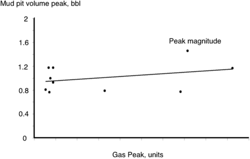
Figure 5.22 Cross-plot of mud pit volume peak versus gas peak corresponding to each conductive natural fracture location identified for Well A-2. Redrawn from Corbeck, 2010.
In absence of other means of validation, patterns in the locations of conductive natural fracture zones between wells were used. Existence of such patterns would confirm tectonic continuities that are essential for history matching of the diagenesis involved to validate the results, because each pair of wells should penetrate similar geologic conditions. Once validated the existence of fractures (or sweet spots), orientation of fractures could be used to refine reservoir characterization. For the case in question, two out of the three parallel well pairs exhibit strong patterns. From visual inspection of the results obtained for Field A, two dominant patterns can be observed, as can be seen in Figure 5.23. A total of seven pairs of natural fractures are aligned at an orientation of roughly N65°E (see Figure 5.24). Only one identified natural fracture from Well A-2 does not have a corresponding feature in Well A-1. For each of the seven natural fracture planes identified, the estimated apertures of the corresponding pair of natural fractures compare well, with the exception of pairs four and five (see Table 5.7).
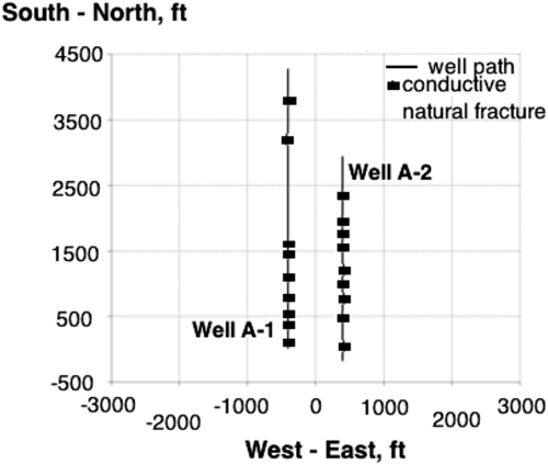
Figure 5.23 Plan view of Field A. Wells A-1 and A-2 are parallel wells drilled in the S–N direction. The lateral spacing between these wells is roughly 800 ft. Redrawn from Corbeck, 2010.
5.6. Reservoir Characterization with Image Log and Core Analysis
As presented in Table 5.1, image logging and core analysis present an important stage of reservoir characterization. Techniques for directly assessing near-wellbore fracture density, fracture aperture, and fracture orientation are presently available to the industry by means of image log testing. Examples of image log techniques include borehole video camera, acoustic formation image technology (AFIT), and resistivity image logs. These three methods are based on different fundamental principles and each has its own set of advantages and disadvantages. A common drawback is that the image resolution quality is generally too poor to be able to identify conductive features that are believed to be on the order of 100-μm wide. Circumferential Borehole Imaging Log (CBIL), when utilized for potential fractured layers already tagged by other techniques (as acoustic waveforms), has been proved as very effective and detailed. Each of the following logs also gives information that can lead to refinement of reservoir characterization.
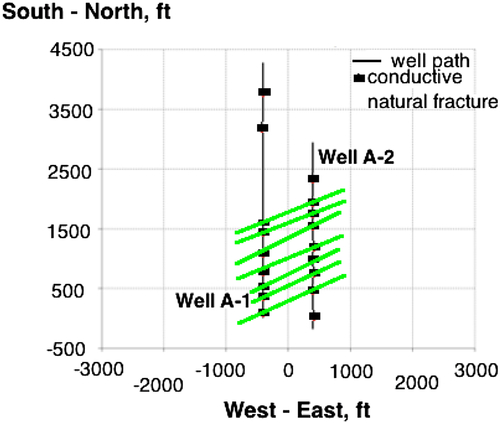
Figure 5.24 Natural Fracture System Orientation #1 for Field A. A dominant pattern exists that seems to indicate the presence of a natural fracture system oriented at N65°E.
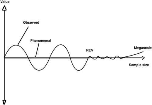
Figure 5.25 Representative elemental volume in fractured reservoirs is greater than core size. Redrawn from Islam et al., 2014.
• Spontaneous Potential
• Gamma Ray Log
• Density Log
• Neutron Log
• Dual-Induction Log
• Sonic Log
Following new array of logs has recently been introduced.
• Array Induction Log
• Array Sonic Log
• Electromagnetic Propagation Log
• Nuclear Magnetic Resonance
One should highlight here that the representative elemental volume (REV) for fractured reservoirs is greater than the core size as well as the depth of resolution of most imaging tools. As can be seen from Figure 5.25, below REV, fluctuations occur. Any correlation that is apparent must, therefore, be corroborated/refined with previously available data, starting from data acquired during geological survey.
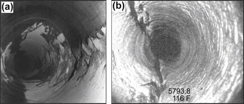
Picture 5.1 (a) Example of borehole breakout taken by a downhole camera. (b) Example of a borehole fracture observed on a downhole camera. Figure 4(b) from Asquith and Krygowski, 2004.
Visual observation with downhole camera is the most effective tool for gathering information on natural fractures. Conventionally, borehole video cameras have been used in oil and gas wells to investigate wellbore integrity, but they have also been utilized for the purposes of natural fracture characterization with limited success. One report by Overbey et al. (1988) presents a horizontal well drilled with air in which borehole video was used to identify fractures. It is important to have a clean borehole so as to facilitate borehole imaging. In this particular study by Overbey et al. (1988), more than 200 features were identified as natural fractures over the 2217 ft of wellbore that was surveyed with the video camera. The report presents an approach to interpret the fracture orientation based on the geometry of the observed feature. The report makes no attempt to quantify the aperture of the features identified or to distinguish between conductive and nonconductive features. The report concludes that borehole video cameras can be implemented as a natural fracture identification technique in air-drilled horizontal wells in low-pressured reservoirs. Optical image logging tools, such as the Optical Televiewer (from Schlumberger) and Downhole Video tool (from Downhole Video), are wireline tools that utilize cameras to directly image the wellbore wall. Picture 5.1 shows such an image.
5.6.1. Geophysical Logs
In general, following geophysical logs are routinely available for reservoir characterization.
• Gamma Ray (GR) Spectralog – this one is based on collecting gamma-ray signals from natural rocks in the reservoir. This log can be performed in open as well as cased holes and allows a detailed stratigraphic reconstruction for the entire depth of the well, even in case of cuttings absence due to total loss of circulation.
• Densilog and Acoustilog—contribute to the stratigraphic structural reconstruction of the well and are essential for the bulk density and seismic wave velocity determination in order to give calibration elements for the interpretation of surface gravimetric and seismic surveys. Furthermore these logs are fundamental to computing the formational elastic parameters and their variations in case of presence of fractures.
• Multiarm Caliper—is very useful not only for the imaging of the hole geometry, but also for structural reconstruction by means of breakout analyses.
• Borehole imaging log—allows the 360° mapping of the walls of the hole by analyzing the formational variation of both velocity and resistivity. This is the only specific tool for the direct fracture analyses in terms of nature and geometric parameters.
Usually, during the field recording phase it is possible to make a preliminary individuation of levels that can be potentially fractured. These are very often associated to:
• sharp decrease of bulk density and P-wave velocity (Vp);
• strong attenuation of the wave form;
• intense and very thin cavings in the walls of the hole;
• peaks of GR in case of mineralized fractures.
Borehole imaging tools provide an image of the borehole wall that is typically based on physical property contrasts. There are currently a wide variety of imaging tools available, though these predominately fall into two categories: resistivity and acoustic imaging tools.
Resistivity imaging tools provide an image of the wellbore wall based on resistivity contrasts (Ekstrom et al., 1987). Resistivity imaging tools consist of four- or six-caliper arms with each arm ending with one or two pads containing a number of resistivity buttons. Resistivity imaging tools provide one with the same information on borehole diameter and geometry as the older dipmeter tools, however, the resistivity buttons also allow high-resolution resistivity images of the borehole wall to be developed. There are a wide variety of wireline resistivity imaging tools available, some of the more common tools are the Formation MicroScanner (FMS; from Schlumberger), Formation MicroImager (FMI; from Schlumberger), Oil-Based MicroImager (OBMI; from Schlumberger), Simultaneous Acoustic and Resistivity tool (STAR; from Baker Atlas), Electrical MicroScanner (EMS; from Halliburton) and Electrical Micro Imager (EMI; from Halliburton). Furthermore, recent years have seen the development of a range of logging while drilling (LWD) or measurement while drilling (MWD) resistivity image logging tools, such as the Resistivity At Bit (RAB; from Schlumberger) and STARtrak (from Baker Inteq). For more details on resistivity image logging tools see Ekstrom et al (1987) or Asquith and Krygowski (2004).
Acoustic tools, on the other hand, emit high frequency sonar waves. The acoustic imaging tool then records the amplitude of the return echo as well as the total travel time of the sonic pulse. The acoustic wave travel time and reflected amplitude are measured at numerous azimuths inside the wellbore for any given depth. These data are then processed into images of the borehole wall reflectance (based on return echo amplitude) and borehole radius (based on pulse travel time). There are a wide variety of acoustic imaging tools available, some of the more common tools are the Borehole Televiewer (BHTV; from Schlumberger), Ultrasonic Borehole Imager (UBI; from Schlumberger), Circumferential Borehole Imaging Log (CBIL; from Baker Atlas), Simultaneous Acoustic and Resistivity tool (STAR; from Baker Atlas), Circumferential Acoustic Scanning Tool-Visualization (CAST-V; from Halliburton) and the LWD/MWD Acoustic Caliper tool (ACAL; from Halliburton).
The use of AFIT has been implemented to characterize the permeability of feed zones in oil and gas and geothermal wells. A description of the AFIT tool is given by McLean and McNamara (2011):
As the AFIT tool is lowered and raised in the well an acoustic transducer emits a sonic pulse. This pulse is reflected from a rotating, concave mirror in the tool head, focusing the pulse and sending it out into the borehole. The sonic pulse travels through the borehole fluid until it encounters the borehole wall. There the sonic pulse is attenuated and some of the energy of the pulse is reflected back towards the tool. This is reflected off the mirror back to the receiver and the travel time and amplitude of the returning sonic pulse is recorded. Through the use of the rotating mirror (≤ 5 rev/sec) 360° coverage of the inside of the borehole wall can be obtained.
In practice, the interpretation of AFIT data is quite sophisticated. Planar natural fractures appear as sinusoids in the imaged data set, as shown in Figure 5.26.
Data processing software allows for characterization of geologic features including strike and dip, fracture aperture, and fracture density. The signal amplitude can be used to distinguish between open and closed fractures. Low amplitude signals are seen as dark features on the acoustic image and often interpreted as open. High amplitude signals are seen as light features on the acoustic image and are thought to be attributed to mineral fill. These high amplitude features are usually considered as closed fractures that do not contribute to flow. While McLean and McNamara (2010) report a good level of correlation between measured feedzone fluid velocity and fracture aperture determined from AFIT, the fracture apertures reported range from several centimeters to greater than 50 cm. This implies that the resolution of AFIT can at best distinguish fractures of roughly 1–2 cm. This is nowhere near the level of resolution quality necessary for fracture characterization in highly fractured tight gas reservoirs.
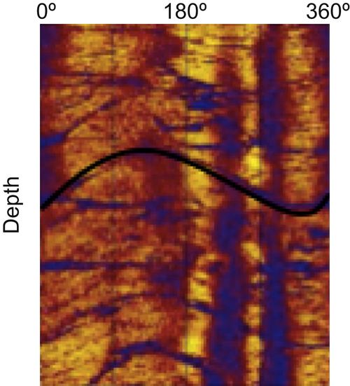
Figure 5.26 Example of an AFIT image log. The horizontal axis is azimuth around the wellbore. The sinusoids are interpreted as planar geologic features. From Mclean and McNamara 2011.
Resistivity image logs, also called FMI logs, have been documented as an improved technique to characterize geologic features along the wellbore. These techniques make use of a tool that places an electrode at constant electrical potential against the borehole wall and measuring the current. Picture 5.2 shows the device. The tool is a small-diameter imaging tool that can be deployed with or without a wireline. The high sampling density of these tools (e.g., 120 samples per foot) provides extremely high resolution in the image quality. Microresistivity imaging tools have the ability to visualize features down to 2 mm in width. Careful interpretation of resistivity image logs can provide helpful information about the geologic conditions near wellbore, including dip analysis, structural boundary interpretation, fracture characterization, fracture description, and fracture distribution.
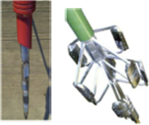
Picture 5.2 Photograph of a microresistivity imaging device (left) passing through drill pipe and (right) in the open position. From Kalathingal and Kuchinski 2010.
Data obtained from all three of these image log techniques can be analyzed to gain useful insight about the natural fracture system and state of stress system near wellbore. Barton and Zoback (2002) present an approach for discriminating natural fractures from drilling-induced fractures from different types of image logs, and using this knowledge to determine the state of stress in situ. It has been well documented that drilling-induced tensile fractures will form in the azimuth of the maximum horizontal principal stress. If the three in situ principal stresses can be determined and the formation fluid pressure is known, then a Coulomb failure analysis can be applied to the natural fractures identified in the image logs. Shear and effective normal stresses acting on each fracture plane can be determined from knowledge of the orientation of the fracture plane with respect to the orientations of the principal stresses. The Mohr–Coulomb failure envelope for fractures is determined from laboratory measurements on prefractured rock. The failure line is constructed assuming no cohesion and using the friction angle of the prefractured rock. Poles to fracture planes are then displayed on the Mohr diagram. Critically stressed fracture planes lie above the Mohr–Coulomb failure envelope (Figure 5.27). Barton and Zoback (2002) report a strong correlation between critically stressed fracture planes and hydraulic conductivity of the fractures. These findings indicate that only a small percentage of the total number of fractures are likely to contribute to flow.
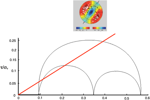
Figure 5.27 These figures illustrate the concept that critically stressed natural fractures predominantly contribute to fluid flow through reservoirs. Redrawn from Barton and Zoback 2002.
5.6.1.1. Circumferential Borehole Imaging Log
Recently, the CBIL, based on the digital acoustic imaging technology (McDouglas and Howard, 1989), has gained popularity among geophysical tools for characterizing fractured formations. All the processing steps are mainly aimed at pointing out all those variations of the rock physic characteristics that can be related to the presence of fracture systems.
The first processing phase involves the Densilog and Acoustilog in order to compute the acoustic impedance, the reflection coefficient, and the synthetic seismogram. The last one is particularly useful for a comparison with surface and well seismic profiles data, because seismic reflections have been proved to be very often a signature of fractured horizons.
The wave form analysis, recorded by means of advanced digital acoustic tool, allows to map the image of the instantaneous amplitude. This shows the wave form energy distribution and content evidencing very clearly that wave form attenuation is due to fractures. Furthermore, the S-wave velocity (Vs) and the Vp/Vs ratio are also computed from the wave form analyses. These parameters are combined with the density values and many elastic properties can be computed (see Figure 5.28). Among these elastic parameters, the fracture toughness modulus is particularly sensitive to the presence of fractured levels.
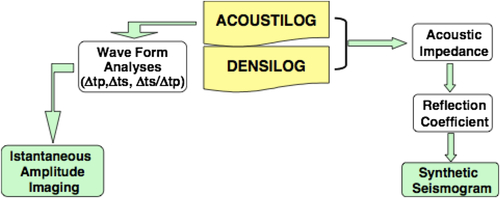
Figure 5.28 Processing flow chart of density and acoustic well logging data. From Batini et al., 2002.
The second processing phase (Figure 5.29) is aimed at the fracture characterization of both the nature and the structural pattern using data from Multiarms Caliper and CBIL (orientation-corrected in case of deviated wells). Rough structural information comes from the breakout analysis of the Multiarms-oriented Caliper that allows the definition of the minimum horizontal stress direction (σ3), which is orthogonal to the fracture planes considering a vertical direction of the maximum stress (σ1).
CBIL data allow detailed structural reconstruction. In the CBIL tool an acoustic transducer, continuously spinning 360° of the walls of the hole, emits an acoustic pulse directed into the formation and records both the amplitude and the travel time of the returning wave. The acoustic amplitude is mainly a function of the acoustic impedance of the formation, so that fractures and their nature (open, mineralized, foliation, etc.) can be clearly evidenced. Even though the depth of penetration is not impressive with CBIL, detection of fractures even at the hole surface is useful and practical for reservoir characterization.
Advanced CBIL processing techniques provide enhanced 360° acoustic amplitude images of the reflected wave. On these images, it is possible to distinguish different types of fractures as a function of both the acoustic impedance variation degree and of their shape and size. These “structural events” can be then picked and all the geometric parameters (i.e., strike, inclination, and dip direction) computed. Correlations can also be made with other data (e.g., downhole camera, gamma ray, geological data) in order to refine lithological data.
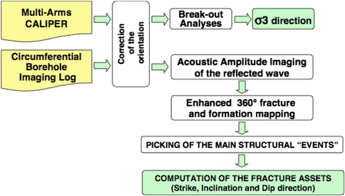
Figure 5.29 Processing flow chart for fracture analyses from well logging.
The most effective way to refine CBIL information is to use it in combination with well test data, which include thermal gradient and injectivity. The utilization of temperature and pressure log can be a useful tool for the identification of each productive zone in the well and the direct measurement of the injectivity. As stated earlier in this chapter, UBD creates a dynamic database. In absence of UBD, similar information can be extracted during an injection test. These test results are affected by the existence of different fractures inside the well, thereby generating data on fracture aspect ratio, density, and others. The temperature profile during an injection test will exhibit a change of slope of the thermal gradient where there is a change in the flow rate, i.e., where there is an adsorbing zone: the thermal gradient is proportional to the fluid that passes in the formation. For a gas well, the thermal change is more intense due to augmented Joule Thomson effect.
The permeability distribution of the reservoir must provide a hydraulic connection throughout all the system; a pressure change in a part of the reservoir (due to exploitation or injection) is propagated in all the system. The propagation velocity of the pressure wave depends on the so-called “hydraulic diffusivity.” The well testing is the way for measuring the most important reservoir parameters, as well as the characteristics of the fluid motion. During the drawdown/injection tests, the pressure gauge is placed close to the productive zone and the pressure change is recorded while the well is operated at constant production/injection rate. From the shape of the curve it is possible to identify the reservoir's unique characteristics: the trasmissivity (the permeability–reservoir height product), the skin factor (the well–reservoir coupling factor), the deviation from the ideal radial flow (storage effects, closed or constant pressure boundaries, linear motion of the fluid along preferential paths).
During an interference test, the pressure change of a given well is recorded, while a drawdown/injection test of another one is performed. This is a very important way for measuring the average characteristics of the reservoir in the volume between the two wells, or for establishing a higher limit of the permeability in the case of negative response.
Batini et al. (2002) presented a comprehensive field case study that utilizes CBIL along with well tests and other geophysical logging. They reconstructed the stratigraphy in order to determine main rock physical properties for each geological formation of interest. Table 5.8 gives an example of geological characterization performed by means of the GR Spectralog, which gives a value of total GR and of its spectral components: Potassium (K), Thorium (TH), and Uranium (U).
Table 5.9 shows some of the physical characteristics of the rock. This is necessary for further analysis of data. They also conducted core analysis on two core samplings within the interval in question. These data can be utilized to refine static data gathered independent of core sampling. The bulk density of 2.6 g/cm3 can be compared with the previous indirect measurement from geophysical logs of 2.77 g/cm3 for the mica schists reservoir rock. Table 5.10 lists these data.
The case study involves a geothermal well that was drilled during May 8, 2000 through September 12, 2000. The formation is cased and the open hole started at a depth of 2202 m. The first important fractured zone has been highlighted at 2600 m; after acidification and hydraulic stimulation an injection test measured a low injectivity: 1.6 m3/h/bar. Subsequently, a T&P = temperature and pressure log has been recorded during another stimulation (with 80 kg/s for 2 5 h), followed by another medium-duration injection test (with 8 kg/s). Three adsorbing zones have been identified, but, due to the low overall injectivity, it was decided to deepen the well, until the final depth of 4002 m was reached. The following tests were performed:
• Build up immediately after drilling;
• A 17-day production test (the well production could be estimated as 4 kg/s at 1.6 MPa well head pressure);
• Two T&P logs during the production test, with an indication of six productive fractured zones (Fig. 5.30);
• An interference test, showing a linear motion connecting the two wells;
• Final build up after production test.
Table 5.8
Geological Characterization from GR Spectralog
| Lithology | Depth interval (m) | GR (GAPI) | K (%) | TH (ppm) | U (ppm) |
| Neogene Sediments | 0–280 | 44.0 ± 3.8 | 1.1 ± 0.1 | 3.9 ± 0.6 | 2.0 ± 0.5 |
| Flysch | 280–550 | 63.0 ± 5.3 | 1.9 ± 0.1 | 2.8 ± 0.77 | 2.8 ± 0.7 |
| Tectonic Wedges | 550–1900 | 48.0 ± 7.6 | 1.92 ± 0.1 | 6.7 ± 1.2 | 2.5 ± 0.7 |
| Phyllites | 1900–2220 | 93.5 ± 12.5 | 2.38 ± 0.6 | 11.7 ± 1.9 | 3.2 ± 1.1 |
| mica schists | 2220–3800 | 109.8 ± 35.5 | 2.40 ± 0.9 | 12.7 ± 4.6 | 4.4 ± 1.6 |
| Gneiss | 3800–4000 | N/A | N/A | N/A | N/A |
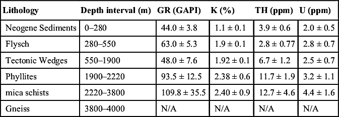
GAPI = gamma ray unit of API (American Petroleum Institute)
Table 5.9
Physical Characteristics of the Reservoir Rock
| Parameter | Value |
| Vp | 4.87 ± 0.32 (km/s) |
| Vs | 2.81 ± 0.20 (km/s) |
| Vp/Vs | 1.7 ± 0.1 |
| Density | 2.77 ± 0.07 (g/cm3) |
| Acoustic Impedance | 12.7 ± 1.6 (km/s g/cm3) |
| Young's modulus | 53.25 ± 10.2 (GPa) |
| Poisson's Coefficient | 0.2 ± 0.06 |
| Fracture Toughness | 0.006 (GPa−1) |
Batini et al., 2002.
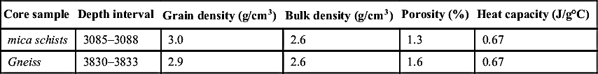
Figure 5.30 shows the temperature profile. Unfortunately, the drawdown analysis does not give a clear indication of the reservoir characteristics, due to the superposition effects of each production zone. The final build-up shows a slight tendency toward a radial motion, with a stabilized flow rate of 2.2 kg/s at 1.6 MPa. Assuming 1000 m of reservoir height, the formation permeability can be estimated as 0.7 mD and a negative skin factor of −4.2. Table 5.11 shows results of the well test.
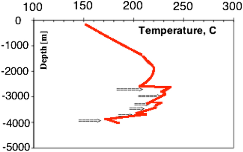
Figure 5.30 Temperature profile shows the existence of a fractured zone. Redrawn from Batini et al., 2002.
The CBIL results gave a means of most definitive confirmation of fractures, as well as quantitative information. The geophysical log processing confirmed that the six depth intervals preliminarily identified for the CBIL investigation were particularly affected by signatures related to the presence of fractures (Figure 5.31).
The CBIL analysis allowed the identification of different kinds of fractures and their geometrical parameters (Figure 5.32). These last were processed and mapped for each interval as “pole density of all the fracture planes,” using the Wulf's lower hemisphere stereographical projection. It should be noted that visual inspection of cores is an integral part of the analysis (last column of Figure 5.32).
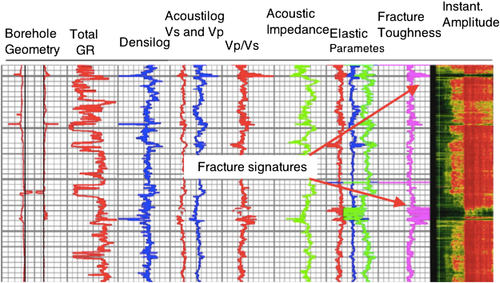
Figure 5.31 Fracture signatures from geophysical logs. From Batini et al., 2002.
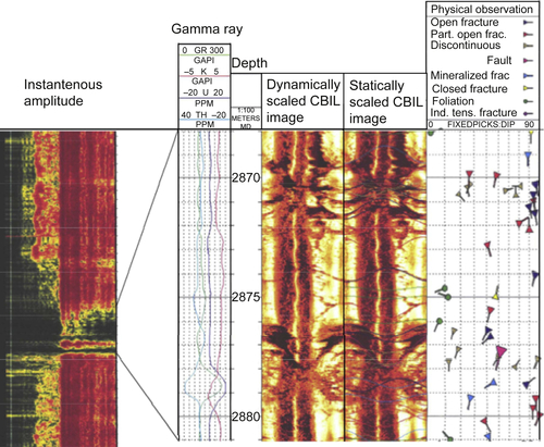
Figure 5.32 Fracture analysis from CBIL. From Batini et al., 2002.
For each interval, the pole density distribution for fractures and faults (foliations excluded) is shown in Figure 5.33 together with the most representative cycle-graphical traces. These are characterized by a prevalent E–W azimuth direction, the dip direction is almost variable, but the inclination shows a tight variation between 65° and 80°.
A comparison with core fracture analysis is possible only for cores extracted from the same metamorphic formation in the vertical well Sesta 6 bis. They are not oriented, so that the only reliable value is an average slope of about 70° measured on few samples of continuous joints.
A comparison between the fractures detected by geophysical logs and well testings is given in Table 5.12 together with a tentative correlation between fracture asset and productivity.
There is quite a correspondence with fractures detected by well testing in four out of six intervals characterized by geophysical fracture signatures. Excluding the deepest productive zone at 3880 m, not investigated by CBIL, the levels with higher productivity (1.77 and 0.33 kg/s) are associated with subvertical fractures (inclination of 70–87°) with an E–W strike direction and northward dip direction.
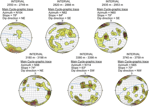
Figure 5.33 Fracture asset mapped as pole density. From Batini et al., 2002.
5.6.1.2. Petrophysical Data Analysis Using Nuclear Magnetic Resonance
Recent years have seen a surge in the use of NMR-based logging tools. It is commonly perceived that NMR alone or in combination with conventional logs as well as special core analysis (SCAL) data can lead to better determination of petrophysical properties of heterogeneous tight gas sand reservoirs (Hamada, 2009). Hamada reported the determination of following parameters of a tight gas formation:
1. Detailed NMR porosity in combination with density porosity, ΦDMR;
2. NMR permeability, kBGMR, which is based on the dynamic concept of gas movement and bulk gas volume in the invaded zone; and
3. Capillary pressure derived from relaxation time T2 distribution, with further possibility of its use in measuring formation saturations, particularly in the transition zone.
Hamada (2009) presented an interesting case study that is used in this section as a template. The case study involves a gas condensate field that produces from a Lower-Mesozoic reservoir. The reservoir is classified as a tight heterogeneous gas shaly sands reservoir. Complex heterogeneity occurs both laterally and vertically due to diagenesis involving kaolinite and illite. As shown in Figure 5.34, the permeability ranges from 0.01 to 100 mD with a narrow band of porosity ranging from 8% to 10%. The petrophysical analysis indicates narrow 8–12% porosity range while wide permeability ranges from 0.01 to 100 mD. This cross-plot is not useful in its original form as there is no discernable trend. Because fractures are not accounted for in the core analysis, any extension of core data to field scale would be severely skewed. Figure 5.34 shows that the cloud points were subdivided into six subunits, ranging from high productivity (green) to very low productivity (black). The integration of NMR analysis as well as SCAL can lead to the establishment of facies-independent porosity and permeability models, thereby avoiding the use of lithology-independent T2 cutoff. Incidentally, lithology-independent cutoff is a standard for conventional reservoir characterization.
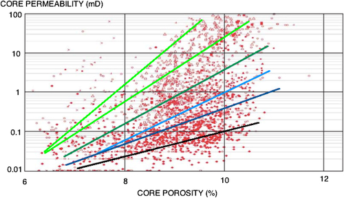
Figure 5.34 Core permeability versus core porosity for a heterogeneous formation. From Hamada, 2009.
Table 5.12
Comparison between Geophysical Logs and Well Testing
| Fractured levels from CBIL | Fracture from well testing | ||||
| Depth (m) | Strike direction | Slop and dip direction | Number of Samples | Depth (m) | Production flow rate (kg/s) |
| 2550–2750 | E–W | 87° N | 242 | 2640 | 1.77 |
| 2820–2890 | E–W | 84° SE | 72 | Not detected | |
| NNW–SSE | 46° E | 22 | |||
| N–S | 50° W | 22 | |||
| 2915–2975 | N–S | 27° E | 36 | 2910 | 0.14 |
| 3180–3210 | E–W | 70° N | 18 | 3240 | 0.33 |
| 3380–3410 | WSW–ENE | 24° SSE | 30 | 3400 | 0.14 |
| 3660 | 0.33 | ||||
| 3730–3780 | Not definable | Few | Not detected | ||
| –––––––Bottom Log––––––––– | |||||
| 3880 | 1.44 | ||||
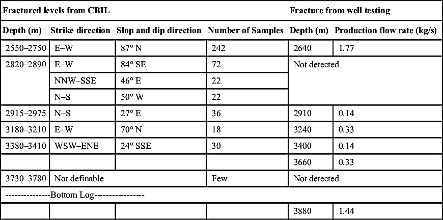
Hamada (2009) presented three-step procedure for integrating NMR data with SCAL and conventional core data. They are:
1. The application of density magnetic resonance (DMR) porosity technique for porosity calculation;
2. Bulk gas magnetic resonance permeability (kBGMR), new technique for permeability calculation beyond the limits of oil-based mud filtrate;
3. Quantify the effect of oil-based mud filtrate on NMR data and then calibration for approximated capillary pressure from NMR.
Freedman et al. (1998) proposed a combination of density porosity and NMR porosity (ΦDMR) to determine gas-corrected porosity formation and flushed-zone water saturation (Sxo). Density/NMR cross-plot is superior to density/neutron cross-plot for detecting and evaluating gas shaly sands. This superiority is due to the effect of thermal neutron absorbers in shaly sands on neutron porosities, which cause neutron porosity readings too high. As a result neutron/density logs can miss gas zones in shaly sands. On the other hand, NMR porosities are not affected by shale or rock mineralogy, and therefore density/NMR (DMR) technique is more reliable to indicate and evaluate gas shaly sands. Freedman et al. (1998) expressed true porosity as:
ϕ=(αβ+α∗ϕD+ββ+α∗ϕNMR)
![]() (5.9)
(5.9)
where ΦD is the apparent density porosity, ΦNMR is porosity determined by NMR, and α and β are given as:
α=(1−(HI)gPg)
![]()
β=ρL−ρgρm−ρL
![]()
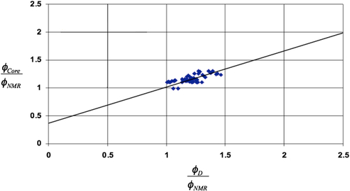
Figure 5.35 Developing filter out of NMR data.
Equation 5.9 can be rearranged as follows:
ϕCoreϕNMR=A∗ϕDϕNMR+B
![]() (5.10)
(5.10)
where A and B can be extracted by cross-plotting core porosity with NMR porosity, thereby, creating a filter that can be used throughout the reservoir. Such cross-plot is shown in Figure 5.35.
Note that at Sgxo = 0, the pores are completely filled with liquid (mud filtrate and irreducible water), so the NMR porosity reading and density porosity should be correct and both should equal to core porosity. As a result, the trend line should intersect at control point, where□ΦCORE/ΦNMR = ΦD/ΦNMR = 1. Fluid density for apparent □ΦD estimation is best fitting at 0.9 g/cc (in this particular case), which is a combination between formation water density and mud filtrate density.
For the above case, A and B are best fitted with the values 0.65 and 0.35, respectively, resulting in the following filter:
ϕDMR=0.65ϕD+0.35ϕNMR
![]() (5.11)
(5.11)
The results of ΦDMR transform applications in the three wells A, B, and C showed very good match between ΦDMR and core porosities as shown in Figures 5.36, 5.37, and 5.38. As a result, it is considered as an independent facies porosity model. These corrected porosities can be used in order to estimate permeability in gas bearing formations.
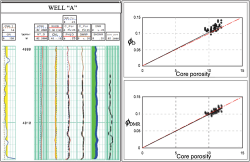
Figure 5.36 Filter for “Well A.” From Hamada, 2009.
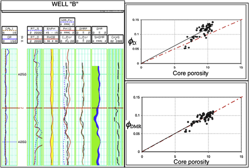
Figure 5.37 Filter for “Well B.” From Hamada, 2009.
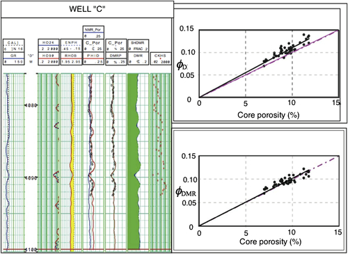
Figure 5.38 Filter for “Well C.” From Hamada, 2009.
Figures 5.36, 5.37, and 5.38 present well logs, showing ΦD and □ΦDMR. Gamma ray and Caliper curves are shown in the first track (GR&CALI); the second track shows depth in meters; the third track shows resistivity; the fourth track shows neutron-density logs; the fifth track shows comparison between core, density, and NMR porosities; the sixth track shows comparison between ΦDMR and core porosity; the seventh track shows saturations of gas (green shadow) and water (blue shadow); and the last track shows core permeability in milliDarcys.
The next step involves correlation with permeability. Bulk gas magnetic resonance permeability (kBGMR) is a new technique for permeability estimation in gas reservoirs. It is a dynamic concept of gas movement behind mud cake as a result of permeability formation, gas mobility, capillarity, and gravity forces. Because gravity forces are constant, capillarity depends mainly on permeability, and mobility depends on permeability and fluid viscosity, which is constant for gas; the gas reentry volume directly function in permeability.
The technique involves:
1. Calculation of gas volume in the flushed zone by using Differential spectrum (ΔTw) Multi acquisition using different waiting times (Tw);
2. Solve diffusivity equation to solve for the volume of gas. Friedman et al. (1998) gave the following expression:
Vg,xo=DPHI−TNMR(HI)f[1−(HI)g∗Pg(HI)f]+λ
Vg,xo = gas volume in the flushed zone
DPHI = formation porosity from density using filtrate fluid density
TNMR = total NMR porosity
(HI)f = fluid hydrogen index
(HI)g = gas hydrogen index
Pg = gas polarization function = 1−exp (−W/T1,g), where W is the wait time and T1,g is the longitudinal relaxation time for gas.
λ=ρf−ρgρm−ρf
![]()
3. Estimate invasion gas saturation, Sgxo with
Sgxo=(ϕD−DMR)∗(ρm−ρL)DMR∗(ρL−ρg)
4. Calculate gas volume approximately by ignoring the gas response in the NMR measurements especially in short Tw, and then the gas saturation in the invaded zone as:
Bulk gas volume (BG) = ΦDMR − ΦNMR
Figure 5.39 shows core permeability versus core porosity. It reflects how the permeability varies between facies to other within same porosity range. The same method is applied for the three wells A, B, and C, and then BG is plotted versus formation permeability, as shown in Figure 5.40. The correlation is normalized by dividing the gas volume by the total porosity of DMRP to be equal to Sgxo, as shown in Figure 5.40.
Sgxo=DMRP−ϕNMRDMRP
![]()
The correlation between Sgxo and permeability shown in Figure 5.41 has resulted in following permeability transform.
KBGMR=0.18∗10(6.4∗Sgxo)
![]()
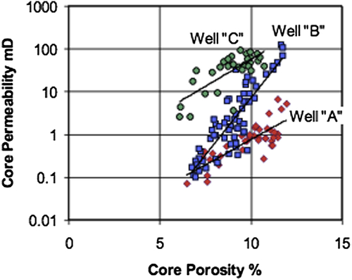
Figure 5.39 Correlation between core permeability and core porosity. From Hamada, 2009.
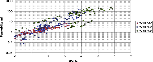
Figure 5.40 Correlation between permeability and BG. From Hamada, 2009.
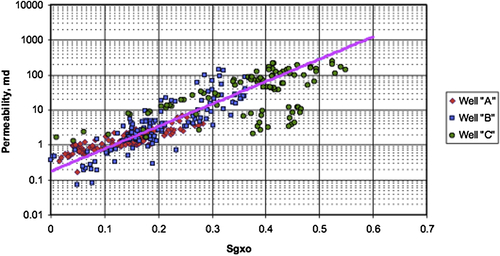
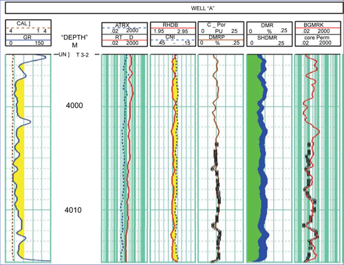
Figure 5.42 Permeability distribution (track 6) for “Well A.” From Hamada, 2009.
Permeability derived using equation 5.11 in the three wells A, B, and C is shown in Figures 5.42 through 5.45. All the three wells A, B, and C show a good match between kBGMR permeability with core permeability.
Similarly, correlation was achieved for capillary pressure by Hamada (2009). Figure 5.44 shows such correlation for “Well B,” reported above.
5.6.2. Core Analysis
The most direct method for characterizing the natural fractures present in the reservoir is to perform core sample analyses. Fracture density and fracture spacing can be determined through visual analysis of the core (e.g., Gale et al., 2007; Kubik and Lowry, 1993). Plugs are typically taken for laboratory experiments to measure permeability and other flow properties. These experiments can only measure an “effective” permeability of the core sample. Generally, it is not possible to determine the natural fracture contribution to flow unless the fracture geometry is well known. The key issue, however, is that experience has shown that using laboratory measurements to represent reservoir-scale properties can be vastly misleading. Nonetheless, engineers are faced with the challenge of interpreting the few available direct measurements of the reservoir rock and translating them to field-scale properties. The idea is to use core data to refine data already collected. In addition, several features, including fracture density, mineralization, fracture opening, shale breaks, etc., can be quantified only with visual inspection.
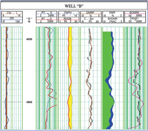
Figure 5.43 Permeability distribution (track 6) for “Well B.” From Hamada, 2009.
Of relevance is also the fact that total porosity can only be determined through core analysis. For unconventional gas perspective, this is of great consequence because as much as 50% recoverable gas can go unaccounted without definitive knowledge of porosity. Conventional assessment of porosity through GR analysis can be vastly misleading in unconventional reservoirs.
Practically all aspects of core analysis are different in unconventional reservoirs from conventional reservoirs. They are highlighted as follows:
1. Low-permeability (matrix and fractures alike) structure itself;
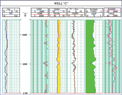
3. Response to overburden stress;
4. Impact of the low-permeability structure on effective permeability relationships under conditions of multiphase saturation;
5. Capillary pressure data as well;
6. The role of fractures and fracture–matrix interactions.
The most prominent of the above is the one related to relative permeability graph. In a conventional reservoir, it is clear that there is relative permeability in excess of 2% to one or both fluid phases across a wide range of water saturation. In traditional reservoirs, critical and irreducible water saturation occur at similar water saturation values. Under these conditions, the absence of common water production usually implies that a reservoir system is at, or near, irreducible water saturation, low-permeability reservoirs, however, one can find that over a wide range of water saturation, there is less than 2% relative permeability to either fluid phase. In these reservoirs, the lack of water production cannot be used to infer irreducible water saturation. In some very low-permeability reservoir, there is virtually no mobile water phase even at very high water saturations. The term “permeability jail” coined by Shanley et al., 2004 describes the saturation region across which there is negligible effective permeability to either water or gas.
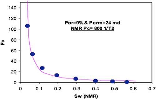
Figure 5.45 Correlation between core Pc (core capillary pressure dots) and NMR Pc (core capillary pressure line).
Low-permeability reservoirs are usually characterized by high to very high capillary pressures at relatively moderate wetting-phase saturations (Figure 5.46). In many cases, wetting-phase saturations of 50% (close to critical gas saturation, Sgc ) are associated with capillary pressures in excess of 1000 psia, suggesting that a large number of pore throats are less than 0.1 μm in diameter and are of the micro- to nanoscale. In many low-permeability sandstone reservoirs, wetting-phase saturation continues to decrease with increasing capillary pressure.
The relationship between relative permeability, capillary pressure, and position within a trap in an unconventional reservoir are shown in Figure 5.47 (Shanley et al., 2004). It shows a reservoir body that thins and pinches out in a structurally updip direction. In this case, significant water production is restricted to very low structural positions near the free water. In many cases, the effective permeability to water is so low that there is little to no fluid flow at or below the free water level. Above the free water level, a wide region of little to no fluid flow exists. Farther updip, water-free gas production is found.
In terms of porosity, overburden pressure plays a significant role in unconventional reservoirs. This is unlike carbonate reservoirs or conventional sandstone reservoirs. Figure 5.48 shows little change in porosity with net increase in stress.
For unconventional reservoirs, such as shale formation, tight sand, etc., porosity is affected by overburden stress. Mechanical compaction is thus an inevitable consequence of burial and basin evolution. Often, this effect is modeled as a function of depth that is most affected by the overburden. However, depth is only a position coordinate that specifies present-day location. Consequently, depth is a poor measure of the processes that have acted upon a sedimentary section through time, which is the primary function that governs all features of a formation. In that sense, everything, including diagenetic process, remains dynamic. Conventional models of shale compaction relate porosity to effective stress using the empirical relationship between void ratio and effective stress established in soil mechanics (Burland, 1990; Yang and Aplin, 2004). Okiongbo (2011) explored the effect of petroleum generation by evaluating the variation in porosity and effective stress in the Kimmeridge clay formation (KCF) above and within the oil window.
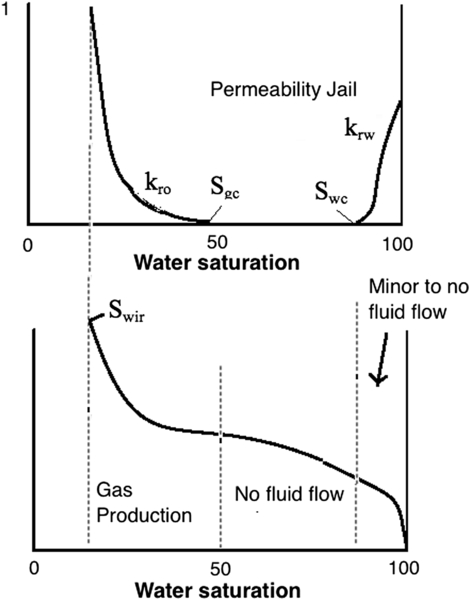
Figure 5.46 Typical relative permeability and capillary pressure curve for an unconventional gas reservoir.
Figure 5.49 shows porosity and effective stress relationship for above and below oil window. A common interpretation of the effective stress–porosity relationship above and within the oil window is that the loss of porosity is faster in the pregeneration zone than within the oil window. In addition, cementation and deeper burial create a relatively stiffer matrix for the KCF sediments within the oil window making it more difficult to compact at high effective stresses. In presence of organic matter, porosity may be impacted by biogenic products. The presence of fractures and fissures alters the dynamics of porosity and pathways for escape of organic gaseous products. The exact nature of the origin of porosity is not known, but there are factors that are not well understood, particularly in the context of unconventional reservoirs. Figure 5.49 also shows a correlation developed by Yang and Aplin (2004) as well as Skempton (1970) and Burland (1990). These models express porosity as a unique function of clay and its natural, fine-grained clastic sediments. Yang and Aplin's (2004) model is based on well data from the North Sea as well as data derived from the studies of Skempton (1970) and Burland (1990). Although the clay content is assumed to be the same (∼65%) in all the data sets, a remarkable difference exists in terms of their organic carbon content. Skempton (1970) and Burland (1990) data sets are low TOC samples (TOC < 1 wt%), the North Sea data set used by Yang and Aplin, (2004) have TOC ranging between 1% and 5wt%, while Okiongbo (2011) data set that are portrayed with red and orange lines have TOC ranging between 5% and 10wt%. In addition, Yang and Aplin's (2004) data set exclude chemically compacted sediments. Above the oil window, the Figure 5.49 indicates similarity between the trend of Yang and Aplin (2004) and that from this study on extrapolation to low effective stresses (<5 MPa). Significant variation only occurs at effective stresses less than five.
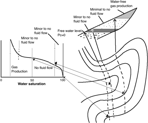
Figure 5.47 Representation of the relationships between relative permeability, capillary pressure, and position within a trap in an unconventional reservoir.
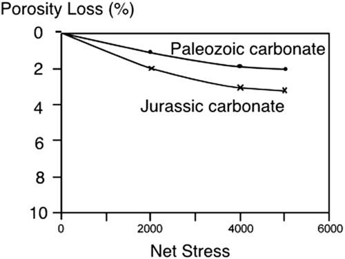
Figure 5.48 Porosity is only slightly affected by net stress for carbonate formations. Data from Lucia (2007) and Hariri et al. (1995).
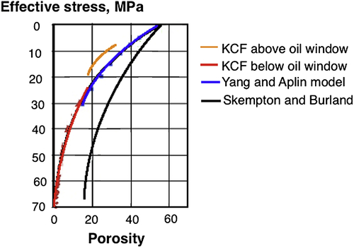
Figure 5.49 Porosity variations with effective stress. After Okiongbo, 2011.
Within the oil window, the Figure 5.49 shows a close agreement between Yang and Aplin's data and Okiongbo data. Overall, the following factors play a role:
• TOC
• Mechanical compaction during diagenesis
• Diagenesis
• Thermal effects
While the first three components have been investigated with some details, thermal effects have not received much attention. Ehrenberg et al. (2009) related geological age of rocks with their diagenesis in order to assess the impact of temperature on porosity. Figure 5.50 shows the effect of geological age on porosity. The impacts of age and lithology are captured in this figure. For petroleum reservoirs, however, the presence of hydrocarbon adds complications. The release of gas increases pore stress, and any escape and migration by hydrocarbon fluids add complications to the nature of porosity. This dependence is different in carbonate formations from silicate formations (including clay and shales). While depth adds to the overburden stress adding to the compaction of pores, it also adds temperature that affects hydrocarbon-bearing pores in a manner different from water-bearing pores. Adds to this is the chemical compaction and cementation that are directly affected by thermal conditions as well as overburden stress.
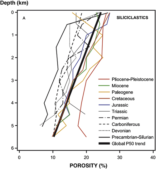
Figure 5.50 Effect of geological age on porosity. From Ehrenberg et al., 2009.
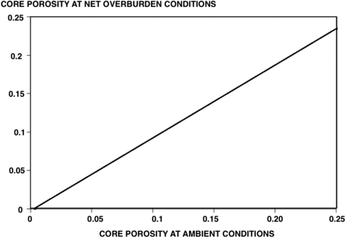
Figure 5.51 Porosity variation under net overburden conditions. Modified from Petrowiki.spe.org.
Figure 5.51 shows overburden stress alone would decrease the porosity. One must caution, however, unconventional reservoirs cannot be modeled uniquely with overburden stress. The degrees of “stress sensitivity” will be a function of the lithology and the pore throat size distributions. Rocks with “slot pores” will be more stress sensitive than rocks with more round pore throats. Slot pores are created by quartz overgrowths during diagenesis. Whenever fractures (natural or induced) are present, the presence of fractures can alter the flow behavior very differently from conventional reservoirs. This has tremendous impact on permeability. Figure 5.52 shows gas permeability at net overburden pressure as a function of gas permeability at ambient pressure (both Klinkenberg corrected). For high-permeability (10–100 mD) core plugs, the permeability under the original overburden pressure is slightly less than the value of unstressed permeability for that same core plug. However, as the permeability of the core plugs decreases, the effect of net overburden pressure on the core plug increases substantially. For the core plugs that had values of unstressed permeability of around 0.01 mD, the values of permeability under net overburden stress were about an order of magnitude lower, or 0.001 mD. The lower permeability rocks are the most stress sensitive because the lower permeability core samples have smaller pore-throat diameters than the higher permeability rocks. As overburden stress increases, the diameter of the pore throat decreases. Because the permeability of a rock is roughly proportional to the square of the diameter of the pore throat, the permeability reduction in low-permeability rocks is much more dramatic than in high-permeability rocks. This behavior would explain the trapping mechanism presented earlier in this section. It also explains why core permeabilities have little relevance when it comes to fractured formations. Figure 5.52 also shows that a fractured formation would show much steeper dependence on overburden stress. This behavior indicates that flow rates would be increased under low stress conditions.
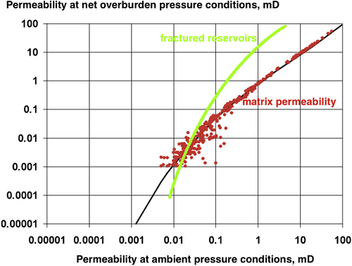
Figure 5.52 Effect of overburden stress on matrix and fracture permeability
5.7. Major Forces of Oil and Gas Reservoirs
There are three main forces prevalent in any petroleum reservoir. They are capillary forces, gravity forces, and mobility forces. It is often useful to study these forces in terms of dimensionless numbers. Three main dimensionless numbers have been identified for many decades. They are capillary number, mobility ratio, and gravity numbers. The interplay of these three numbers is the essence of oil and gas recovery. In 1980s, another number, which is a modified form of “mobility ratio” has been introduced by Peters and Flock (1981) and Bentsen (1978).
Capillary number, Nc is defined as:
Nc=νμσ
![]()
The following formula is also valid:
Nc=k(Δρl)σ

Where:
μ → Displacing fluid viscosity
ν → Darcy's velocity
σ → Interfacial tension (IFT) between the displacing and the displacing fluids
k → Effective permeability to the displaced fluids
Δρl → Pressure gradient
The denominator would contain the term cos θ, where θ is the contact angle, which is a function of rock wettability to certain fluids. The capillary number shows what can be done in a reservoir, the idea being to maximize its value so that more irreducible oil can be recovered. Figure 5.53 shows how capillary number is linked to residual hydrocarbon saturation. Note that x-axis is in log scale. This trend means that Nc has to be increased several orders of magnitude before any impact on residual oil saturation is invoked. However, for unconventional reservoirs, residual saturation bears a different meaning. These reservoirs can be exploited continuously by increasing Nc. Figure 5.54 shows some of the correlations reported in the literature. This graph is also valid for gas reservoirs and is of significance in unconventional reservoirs, where trapping of gas is the main mechanism of gas saturation.
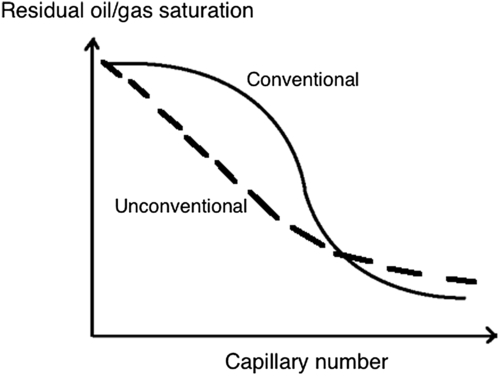
Figure 5.53 General trend of Nc versus residual saturation.
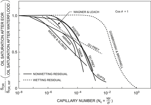
Figure 5.54 Several correlations between capillary number and residual oil saturation.
The above equation shows that in theory the displacing phase viscosity alone will increase Nc. If the increase is manifold, this increase will be sufficient to decrease the residual oil saturation. For instance, by using polymer the displacing phase viscosity can be increased some 1000 fold. This would explain why in laboratory scale, polymer injection has yielded high recovery efficiency. However, large increase in aqueous phase leads to lowering of injectivity. This can be severe for reservoirs that need enhanced oil recovery (EOR), hence creating a dilemma for operators.
The next component that can be manipulated is the Darcy velocity. However, the extent of increase of this velocity is limited due to the fact that flow instability in porous media can be triggered with high displacement rates, causing early breakthrough. In fact, Bentsen's work from 1980s shows that the following relationship exists between instability number (which includes Darcy velocity) and breakthrough recovery. Figure 5.54 shows such correlation. Note that at very low velocity, capillary forces dominate and very little oil is recovered because of the travel of injected water through water films in the porous media. This velocity is unrealistic in field applications and has been demonstrated only in laboratory models. Figure 5.55 shows how a balance between viscous and capillary forces leads to the formation of stable and stabilized front. This segment has the highest breakthrough oil recovery. This segment corresponds to the classic Buckley–Leverett profile. Practically all laboratory models are operated at this regime. For instance, unsteady state relative permeability measurement is performed using flow rates that would correspond to this flow regime. This fact is heavily consequential as none of these relative permeability graphs applies to a flow regime other than stable and stabilized. In case the flow regime is unstable, viscous forces dominate the process and early breakthrough takes place. As the instability number is increased, the breakthrough recovery declines. For very high instability number values, however, the decline is arrested and breakthrough recovery becomes insensitive to instability number.
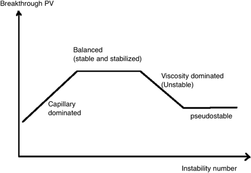
Figure 5.55 General trend of breakthrough recovery and instability number.
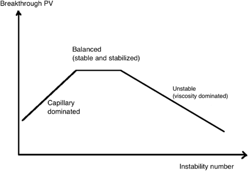
Figure 5.56 Instability number versus breakthrough recovery for immiscible gas injection.
For gas injection, laboratory models and theoretical interpretation thereof show that a different trend emerges. This is shown in Figure 5.56. Note that the stable region is very small and the unstable region is extended to very large instability numbers. The pseudo-stable region is missing within practical limitations of instability numbers.
In general, it is understood that increasing velocity of displacement is not an option for reducing residual oil saturation or increasing recovery through EOR. However, the support for this conclusion came much later than the original conclusion. Until now, the science of instability is little understood. The science of scaling up laboratory results of such cases is in its infancy.
The next factor considered is IFT. Reduction of IFT is at the core of all chemical flooding techniques. For perfect miscibility, the IFT is reduced to zero, signaling total recovery. However, such is never the case in the reservoir. Even when the operating conditions (e.g., injection pressure greater than minimum miscibility pressure) are met, natural media does not offer conditions conducive to instant or perfect miscibility. There is always a transition zone for which the concentration of each component goes through a gradient.
It is conventionally known that if miscibility conditions prevail, the recovery is very high, even if perfect miscibility is not achieved. The most important condition, however, is the stability of the displacement front. Stability was historically connected to mobility ratio, given by the following equation.
M=λing/λed,
![]()
Where:
λing → Mobility of the displacing fluid, (kingμing)
λed → Mobility of the displaced fluid, (kedμed)
Several authors studied the relation between capillary number and residual oil saturation that is presented in the Figure 5.54. Thus, the significant increase in oil/gas recovery was due lowering the IFT between the fluids and pressure gradient promoting a reduction in the capillary number.
Since mobility ratio is less than one (M < 1), the displacement is stable, a fairly sharp “shock front” separates the mobile oil and water phases, and the permeability to water stabilizes fairly quickly. In other case, where the mobility ratio is slightly greater than one (M > 1) is considered unfavorable, because it indicates that the displacing fluid flows more readily than the displaced fluid (oil), and it can cause channeling of the displacing fluid, and as a result, bypassing of some of the residual oil. Under such conditions, and in the absence of viscous instabilities, more displacing fluid is needed to obtain a given residual oil saturation. However, if the value is close enough or equal to unity, the displacement is nearly pistonlike, and is denoted by a favorable mobility ratio. Mobility ratio influences the microscopic (pore level) and macroscopic (areal and vertical sweep) displacement efficiencies.
For waterflood, it is M that is the unique function comes from Buckley–Leverett.
The mathematical relationship between microscopic and macroscopic recoveries efficiencies are represented using the oil recovery factor (Rf), and it can be given by the following formula:
Rf=Ev×Eh×Em
![]()
Where:
Em=EI(SoI−Sor)
The macroscopic sweep efficiency is defined by the horizontal and the vertical sweep efficiencies. The horizontal sweep efficiency is related to the mobility ratio and the vertical sweep efficiency depends on viscous to gravity forces ratio. The vertical sweep efficiency is related to difference in density of the injected fluid and in situ fluid. From early days on, there have been efforts to relate recovery efficiency to mobility ratio. However, until 1980s, it only considered mobility ratio as a unique function of recovery efficiency. While this is a simplistic representation, this was the only correlation available for decades. Until now, many operators use this correlation in order to design both waterflood and chemical flood projects. Figure 5.57 shows one such correlation. This equation is a deduction from Buckley–Leverett equation that shows the following relationships to hold. Here fw and fo are fractional flow of water and oil, respectively.
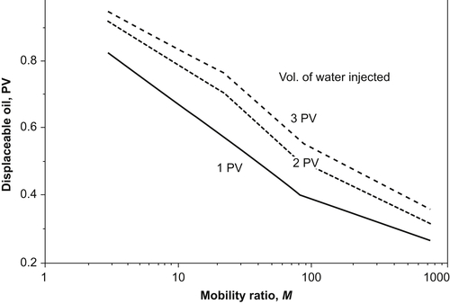
Figure 5.57 Correlation of mobility ratio with oil recovery for waterflood.
fo=11+M,fw=11+1M
![]()
The idea is to manipulate the injection fluid viscosity or mobility in order to maximize oil recovery potential. This correlation does not include the effect of viscous fingering. Such fingering is a possibility when the mobility ratio is greater than one, unless there is a gravity advantage to the injected fluid. For instance, if a gas is injected from structurally higher locations, it would stabilize the displacement front. This phenomenon was long recognized but not included in a dimensionless number until the early works of Flock and Bentsen. Even after these pioneering works, the petroleum industry continued to use older version that included capillary number, Nc, concept or its variation to delineate the onset of fingering. For instance, see the following equation outlined by Lake (1989)
NL=(ϕK)1/2μwυLkrweσcosθ
The above criterion was applied by several researchers and all determined that this definition of instability is grossly insufficient. A far better set of results were obtained using Peters and Flock (1980) criteria. Peters and Flock (1980) worked with velocity potential to come up with a stability criterion for a cylindrical system. It was for immiscible fluid and for the first time they introduced a variable that contains the dimension of the reservoir (or model thereof). It meant, the same system that would show no fingering in lab scale will show fingering in field scale. While in chemical engineering the dimension is always incorporated in determining stability of flow in an open duct, for petroleum reservoir applications it was new. For petroleum reservoirs, the characteristic dimension has always been considered to be pore diameter and not the reservoir dimensions.
Peters and Flock performed a stability analysis of the equations of two-phase flow to determine under what conditions viscous fingers tend to grow and propagate through a porous medium during immiscible flow. Bartley and Ruth (2002) conducted a series of experiments and demonstrated that Peters and Flock's number correlate broadly with their experimental observation of water breakthrough and none supported the criterion offered by Lake (Figure 5.58).
No such correlation existed in terms of capillary number or the modified capillary number as proposed by Lake. See Figure 5.59.
Note that the work of Peters and Flock is based on the earlier theoretical work of Chuoke et al. (1959). Values of the Peters and Flock number, Ns, that are less than 13.56 indicate stable displacements, and values of Ns greater than 13.56 indicate unstable displacements, meaning viscous fingering occurs. The Peters and Flock stability number depends on the mobility ratio, M, a wettability number, Nw, and a calculated value for a characteristic velocity, Vc. In the context of Peters and Flock's work, “stable” means that extensive viscous fingers do not form during a waterflood, or they become damped out; “unstable” means that viscous fingers continue to grow and propagate through the porous medium. They do not include gravity effects. It turns out as a significant omission and would form the basis for modification of the theory and the approach by Bentsen (1978).
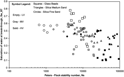
Figure 5.58 Correlation between breakthrough recovery and Peters–Flock stability number.
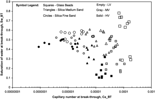
Figure 5.59 There is no correlation between capillary number and water breakthrough.
In this process, fractures play an intermediary role. Older theories did not include the role of macroscopic dimensions and considered pore geometry only. Later theories considered macroscopic dimensions but did not include the role of fractures. Saghir and Islam (1999) showed through a series of theoretical work that fractures are important because they trigger instability. Because conventional theories do not distinguish between fracture dimension and pore geometry and interplay thereof, the role of fracture is ignored. This aspect will be discussed in latter sections.
Bentsen (1978) developed a different instability criterion based on force potential as applied on a rectangular system. He introduced the concept of pseudo-capillary pressure. Both these criteria have gravity numbers in them. Following is the expression developed by Bentsen (1978).
Isr=μwν(M−1−Ng)kwrσe×M5/3+1(M+1)(M1/3+1)24L2xL2yL2x+L2y
Where Ng is the gravity number defined as:
Ng=Δρgkorcosαμoν
![]()
Note that for a vertical injection Ng assumes the largest value possible. In case Ng is larger than the expression, (M−1) the displacement is unconditionally stable. This one shows the value of a gravity-stabilized displacement process that occurs when gas is injected from the top or water is injected from the bottom. This is the case for both miscible and immiscible displacement processes.
In the above expression, σe is the pseudo-IFT, which is:
σeC1σcosθϕ=2−ν1−νˉdAc.
![]()
Ac is the area under the capillary pressure curve and ν is a parameter dictated by the curvature of the capillary pressure.
Many enhanced oil recovery schemes involve the displacement of oil by a miscible fluid. If a scheme is not stable, miscibility cannot occur and all design criteria fail. Stability criteria for miscible processes were developed by Chuoke et al. (1959) but were not modified until Peters and Flock (1980) extended that theory to immiscible displacement processes. Whether a displacement is stable or unstable has a profound effect on how efficiently a solvent displaces oil within a reservoir. That is, if viscous fingers are present, the displacement efficiency and, hence, the economic return of the recovery scheme is seriously impaired because of macroscopic bypassing of the oil. As a consequence, it is of interest to be able to predict the boundary that separates stable displacements from those that are unstable.
Coskuner and Bentsen reported a series of stability numbers that deal with miscible displacement. They used linear perturbation in order to obtain the scaling group. The new scaling group differed from those obtained in previous studies because it had taken into account a variable unperturbed concentration profile, both transverse dimensions of the porous medium, and both the longitudinal and the transverse dispersion coefficient.
It has been shown that stability criteria derived in the literature are special cases of the general condition given here. The stability criterion is verified by comparing it with miscible displacement experiments carried out in a Hele-Shaw cell. Moreover, a comparison of the theory with some porous medium experiments from the literature also supports the validity of the theory. The stability criterion is given below.
UdμdC−kgdρdCsinγˉμD∂ˉC∂xL2Ω·[(1Ω+D′D)(1Ω+1)]−1>π2,withΩ=L2(B2+H2)B2H2(foratwo-dimensionalsysteminwhichH=0,Ω=L2B2)and
Where U = displacement velocity
μ = viscosity of mixture
ρ = density of mixture
C = injectant concentration
k = permeability
g = gravitational acceleration
γ = dip angle
Φ = porosity
Picture 5.3 shows general shapes of viscous fingering in a porous medium. Note that all fingers have similar shape at the onset. As a finger starts to propagate, a dominant one moves faster than the rest of the fingers, leading to bypassing of oils and early breakthrough. This feature is not included in conventional analysis.
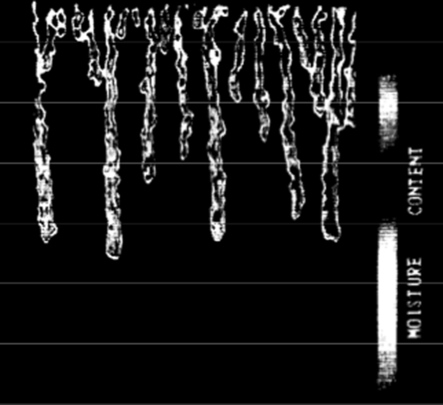
Picture 5.3 Viscous fingering in a miscible displacement process.
When it comes to miscible flood, a mixed scenario of immiscible and miscible displacement processes emerges. It is because every reservoir contains water and an immiscible process is inherently present. This fact is best utilized in designing water alternated with gas (WAG) processes that minimize the use of expensive chemicals. One such example is CO2 miscible injection. Figure 5.60 shows the predominant displacement fronts in a typical CO2 WAG injection process.
Note how the displacement front between oil and miscible gas is likely to be unstable because of the unfavorable mobility ratio, whereas the displacement front between water and miscible gas (CO2 in this case) is likely to be stable. This is one of the greatest advantages of WAG that is often overlooked. In addition, WAG makes it possible to access different segments of trapped oil, as the wettability natures of gas and water are different. The combination of two different types of flooding has other advantages as well.
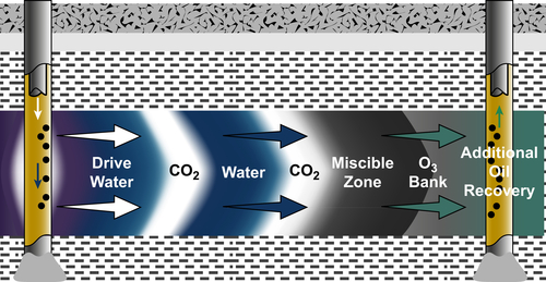
Figure 5.60 Typical CO2 WAG process.
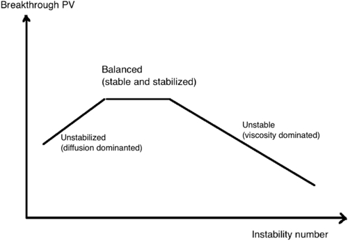
Figure 5.61 Breakthrough recovery versus instability number for miscible flood.
Figure 5.61 shows overall trends of breakthrough recovery with instability number for miscible flood processes. This is a theoretical graph. However, field results as well as scaled laboratory results indicate that this is prevalent. The number for which stability breaks down is important and is generally elusive. All theories are simplified and in need of adjustments due to heterogeneity of the formation. While instability numbers have such components as reservoir dimension and permeability, no one yet added a coefficient that would include heterogeneity in the equation. Yet, most candidates for miscible injection are heterogeneous.
It is likely that the graph moves toward the left for fractured formations and toward the right if those fractures are plugged. This can be corrected if the permeability of the reservoir is filtered and is representative of the reservoir. This aspect will be discussed in a later section.
The Capillary number expression shows lowering the IFT and/or increasing the contact angle will increase the capillary number. This is the basis of chemical as well as gas injection (along with various types of gas/water injection). Through the injection of a chemically active fluid, the IFT of the displacement front is decreased, leading to the recovery of residual oil. On the other hand, if rock wettability is changed, similar impact of lesser intensity can occur.
The property of a fluid is directly related to the viscosity of crude oil within the reservoir. These properties are determined by standardized laboratory procedures. Unfortunately the test results do not represent a general characteristic of the reservoir, because the samples are taken from different sites within the reservoir. The prediction of the reservoir fluid properties becomes even more complex when the prevailing conditions within the reservoir change as a result of undergoing processes, leading to unexpected reaction during injection and production operations.
Variations in rock–fluid interaction with changing conditions in a reservoir result in wettability variations, which in turn affect flow parameters such as capillary pressure and relative permeability, affecting both dynamic recovery as well as ultimate recovery from such reservoirs.
Figure 5.62 shows how end-point permeability values affect residual oil saturation. This figure shows how the use of different gas as well as WAG can affect the ultimate recovery.
For the dynamic part of the displacement process, the most profound impact is through alteration of permeability graphs. Figure 5.62 shows some examples of how lowering of IFT alters effect permeabilities of both water and oil. The permeability values corresponding to lowest IFT form straight lines. While this is true in a core flood test, it rarely occurs in the field and discrepancy between laboratory data and field results emerges. In reservoir simulation studies, it has been demonstrated that the oil recovery with straight line permeability curves do not show an oil recovery curve markedly better than others. This happens even after one overcomes the stability problem that occurs when such straight lines are assigned as relative permeability values of an immiscible system (e.g., oil and gas).
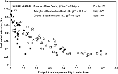
Figure 5.62 End-point relative permeability correlates with residual oil saturation.
The most frequently encountered saturation end points are as follows:
• Residual oil saturation
• Irreducible water saturation
• Trapped-oil and trapped-gas saturations
• Critical gas and condensate saturations
Residual oil, irreducible water, and trapped-gas and trapped-oil saturations all refer to the remaining saturation of those phases after extensive displacement by other phases. Critical saturation, whether gas or condensate, refers to the minimum saturation at which a phase becomes mobile.
The end-point saturation of a phase for a specific displacement process depends on the following:
• The structure of the porous material
• The wettabilities with respect to the various phases
• The previous saturation history of the phases
• The extent of the displacement process (the number of pore volumes injected)
The end-point saturation also can depend on IFTs when they are very low and on the rate of displacement when it is very high. For unconventional gas reservoirs, lowering of IFT, any chemical treatment, any thermal alteration, or onset of fractures, leads to the alteration of relative permeability graphs. Figures 5.63 and 5.64 shows how such movement can translate into gas production.
Results reported by Chatzis et al. (1983) give general insight on the combined effects of wettability and porous structure on residual saturations. In tests with an unconsolidated sand of nonuniform grain size, the wetting phase (oil) was displaced by a nonwetting phase (air) from an initial saturation of 100% to a residual value. In general, it is known that
• Residual saturation of a wetting phase is less than the residual saturation of a nonwetting phase.
• Residual saturation of a nonwetting phase is much more sensitive to heterogeneities in the porous structure.
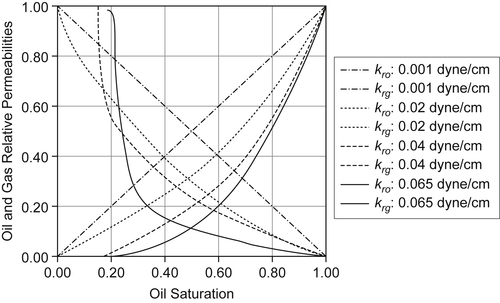
Figure 5.63 Relative permeability curves are altered by lowering of interfacial tension.
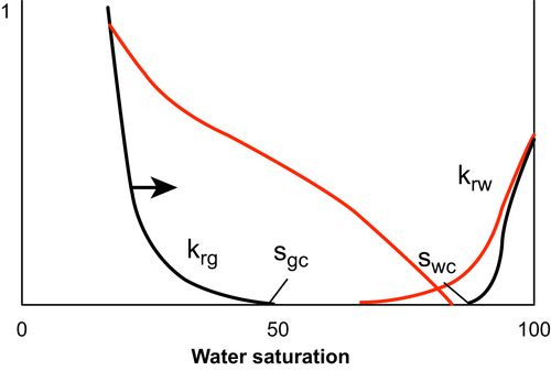
Figure 5.64 Permeability jail can be removed with thermal or chemical alteration in an unconventional reservoir.
General conclusions on the effects of wettability are useful, but the diverse array of wetting alternatives suggests caution, especially in oil/water reservoir systems. This wide range of wetting possibilities is an obstacle to interpreting or predicting the effect of wettability on end-point saturations. Indeed, conflicting results for different porous media are likely to occur. For example, Jadhunandan and Morrow (1995) report that residual oil saturation displays a minimum value for mixed-wet media as wettability shifts from water-wet to oil-wet—contrary to the results of Bethel and Calhoun (1953) that reported a maximum for media of uniform wettability.
For gas reservoirs, such analysis is important because of the critical gas saturation. The critical gas saturation is the saturation at which gas first becomes mobile during a gas flood in a porous material that is initially saturated with oil and/or water. If, for example, the critical gas saturation is 5%, then gas does not flow until its saturation exceeds 5%. Values of Sgc range from 0% to 20%. For gas condensate reservoirs, this is of utmost importance. Interest on the mobility of condensates in retrograde gas reservoirs developed in the 1990s, as it was observed that condensates could hamper gas production severely in some reservoirs, particularly those with low permeability. The trend of increasing critical condensate saturations with decreasing permeability, as summarized by Barnum et al., (1995), is reproduced in Figure 5.65.
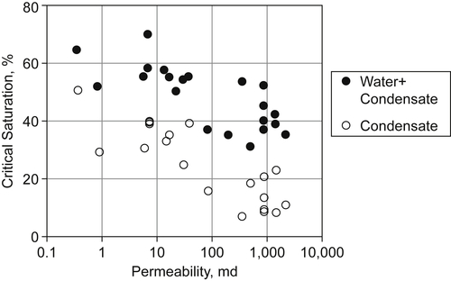
Figure 5.65 Critical gas saturation for various permeability values of a gas condensate reservoir.
This information is important for designing of WAG processes. The WAG ratio can also be defined as the ratio of the volume of water injected within the reservoir compared to the volume of injected gas. It plays an important role in obtaining the optimum value of the recovery factor corresponding to an optimal value of the WAG ratio. This optimal WAG ratio is reservoir-dependent because the performance of any WAG scheme depends strongly on the distribution of permeability as well as factors that determine the impact of gravity segregation (fluid densities, viscosities, and reservoir flow rates). Studies made by John and Reid (2000) showed that the WAG ratio strongly depends on reservoir's wettability and availability of the gas to be injected. When the WAG ratio is high, it may cause oil trapping by water blocking or at best may not allow sufficient solvent–oil contact, causing the production performance behave like a waterflood. On the other hand, if the WAG ratio is very small, the gas may channel and the production performance would tend to behave as a gas flood, the pressure declines rapidly, which would lead to early gas breakthrough and high declination on production rate. To find the optimal WAG ratio, it is necessary to perform sensitivity analysis, proposing different relations of WAG ratio to study the effect on oil recovery.
Even though enhanced gas recovery has not been applied in the field at a commercial level, the fundamental mechanisms show that an enhanced gas recovery scheme is more useful and more likely to be successful than pressure maintenance or waterflood. It is because injected gas is less prone to creating channels or fingers in a gas reservoir than an oil reservoir. In addition, miscibility can be achieved in a gas reservoir under easily achievable conditions. Finally, the use of waste gas or gas that would be otherwise flared makes the economics of the project quite appealing.
5.8. Reservoir Heterogeneity
The degree of interconnection between the pores of an oil reservoir, are rarely evenly distributed due to nonuniformity of pore size, which gives rise to disordered and complex reservoir fluid flow behavior. Geologically speaking, this is known as phenomenon of heterogeneous permeability that can manifest different individual layers, forming different homogeneous layers within the oil reservoir with different permeability values.
Most consolidated formations are highly fractured under reservoir conditions. While the presence of fractures makes them ideal for oil and gas recovery because of very high permeability, the fractures are sealed with secondary cementing activities. Minor porosity of secondary origin occurs locally in sandstones and resulted from the removal of authigenic mineral cements and, to a lesser extent, detrital framework grains. In carbonate-cemented samples, evidence of dissolution includes corrosive contacts between successive carbonate phases and relict cement in pores. Carbonate dissolution features also are observed along the margins of some fractures. Collectively, the dissolution features in sandstones indicate that carbonate cements were previously more widespread before they were partially to extensively dissolved.
Most consolidated formations have fractures in both macroscopic and microscopic scales. Vast majority of these fractures are open without secondary mineralization (Pictures 5.4 and 5.5). The aperture widths commonly exceed 30 μm. One such example is shown in Picture 5.6.
An important characteristic of these fractures is that they typically form a dense network that is highly visible on wetted, slabbed rock surfaces, if the host sandstones and siltstones have high residual oil saturations (Picture 5.7). Such fractures are generally absent in rocks that have little or no residual oil. Often, factures are V-shaped and occluded with pyrite and fine- to coarse-crystalline calcite cement. These fractures, which tend to be small, resemble fluid-escape structures. Such cementation with quartz and cancite (Picture 5.6) can lead to lowering of permeability below the matrix permeability. These types of formations exhibit productivity (or injectivity) lower than one would expect from core and log analysis.
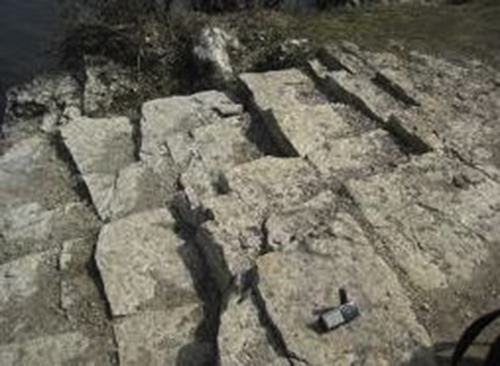
Picture 5.4 Outcrops often show how fractures must be prevalent in consolidated reservoir formations.
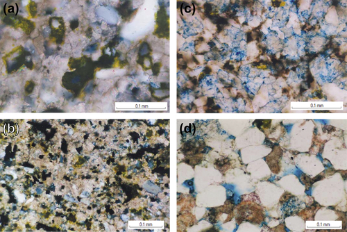
Picture 5.5 Thin section photomicrographs of sandstones illustrating, (a) occurrence and distribution of K-feldspar grains (stained yellow); (b) disseminated pyrite (dark grains); (c) bitumen (opaque material) filling pores and permeating matrix; and (d) secondary intergranular porosity with relict carbonate cement.
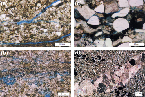
Picture 5.6 Thin section photomicrographs of sandstones depicting, (a) open (noncemented), discontinuous fractures parallel to bedding. Such fractures are abundant and form a pervasive network in sandstones adjacent to mature shales; (b) secondary porosity associated with horizontal fracture swarms; (c) microscopic fractures cross-cutting framework quartz grains. Note bitumen filling secondary intergranular pores; and (d) calcite cemented vertical fracture.
The presence of secondary cementing activities make the porosity–permeability correlation skewed away from matrix permeability. It is, however, the matrix permeability that is routinely reported in core tests. For a fractured formation, matrix permeability has little to do with permeability of the reservoir. The permeability having a dimension of L2, a correlation between permeability and porosity turns out to be linear, as long as the porous medium is homogeneous. This linearity no longer holds if the formation is fractured, as shown in Figure 5.66. If the fractures are open, the medium will have markedly higher permeability than the porosity correlation would indicate. This is consequent because log analysis is usually performed in order to determine point porosity of a core. This is later transformed into permeability values using one of numerous correlations available in the literature. Once the transformation is performed, little attention is paid to the origin of these permeability values. Similarly, core tests as well as specialized core tests are performed on the homogeneous section of the core, leading to the determination of petrophysical properties that have little relevance to the reservoir. Figure 5.66 shows a typical correlation between porosity and log (permeability) of a homogeneous formation as compared to the ones that have fractures. An open fracture increases the reservoir permeability drastically, particularly for median porosity range. On the other hand, this trend is reversed if the fractures are closed due to secondary cementing phenomena.
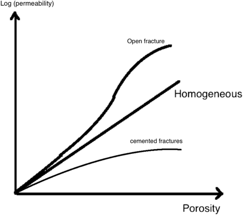
Figure 5.66 Permeability versus porosity correlation depends largely on the nature of heterogeneity.
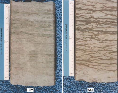
Picture 5.7 Slabbed sandstone displaying reticulated fracture network on wet surface. Note that the permeable nature and distribution of fractures are not apparent when surface is dry.
In terms of anisotropy, it can be invoked due to the presence of fractures. Particular orientation of fractures would skew the directional permeability and the magnitude would depend on the aperture size, secondary cementation, and aperture length. Vertical permeability is affected by the extent of vertical fractures and whether they are open or cemented.
Figure 5.67 shows how porosity is correlated with permeability for various types of formations. Figure 5.68 adds correction factors as a function of fracture frequency. This graph applies to open fractures.
Figure 5.69 shows the trend of vertical permeability (kv) over horizontal permeability (kh) with fracture frequency. While fracture frequency is an important factor in determining the anisotropy, the nature of fractures is crucial for determining magnitude of the permeability ratio. When hundreds of wells and square kilometers of area are considered in order to estimate flow from reservoirs containing billions of barrels, the accuracy of kv/kh analysis can mean a difference of millions of dollars every day throughout the production history.
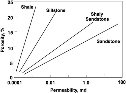
Figure 5.67 Correlation of porosity versus permeability for various types of formation.
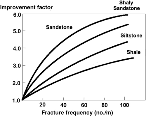
Figure 5.68 Improvement factor due to open fractures.
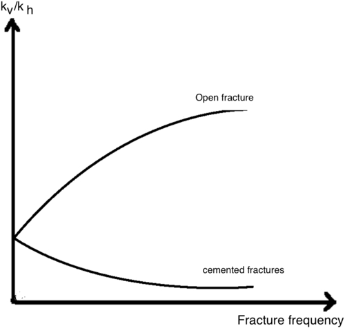
Figure 5.69 The effect of fractures on kv/kh.
The effects of stratification and heterogeneity can be distinct in different reservoirs, affecting various parameters such as capillary pressure, relative permeability, and mobility ratios. The presence of anisotropy and heterogeneity in a reservoir affects the displacement of the native fluids by the injected fluid. Channeling of the solvent through high-permeability regions reduces the storage and displacement efficiency of the displacing solvent. In addition, it can offset viscous fingering through perturbation in case the mobility ratio is not favorable or gravity stabilization is not a dominant mechanism. In case, WAG is being considered, heterogeneity and anisotropy become the most dominant factors that affect oil recovery. It is so because they control the injection and sweep patterns, as well as vertical and areal sweep, viscous fingering, gravity stabilization, and dispersive forces. In addition, horizontal wells play a role different from vertical wells and all calculations pertaining to vertical wells become irrelevant.
In terms of EOR, heterogeneity has tremendous impact. To begin with, the location of trapped oil and the critical capillary number for mobilization of trapped oil would be different for different pore distribution, which is controlled by fracture characteristics of a reservoir. Figure 5.70 shows how different residual saturations would emerge for different pore distribution.
In order to include the influence of fracture and fracture distribution, one must characterize fractures properly. It involves determining frequency and orientation of prominent fractures as identified through examination of cores, micrologs, etc. Commercial software can be used to analyze typical fractures observed in FMS (electrical Formation MicroScanner), as shown in Picture 5.8.
In order to quantify the role of fracture, a rose diagram should be plotted for open fractures. If there is trend for closed or cemented fracture, it should be included in the analysis. It is ideal to develop correlation that is specific to a field.
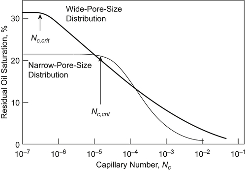
Figure 5.70 Pore size can be affected by fracture distribution and thereby impact residual oil mobilization.
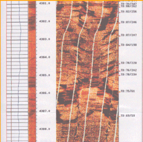
Picture 5.8 Commercial softwares can help identify fractures in FMS logs.
An example of the rose diagram is shown in Figure 5.71. It is a plot with each grouping of data being a petal of the rose. One starts the plot from a center point and draw a line outward (compass direction using a protractor) a distance that matches the number of recorded joints. Rose diagram includes both frequency and orientation with the assumption that all fractures have the same dimension. The rose diagram gives one the dominant orientation of fractures. This is of utmost importance in designing injection production strategies. It is useful to catalog core data, along with microlog information for each well. This information, then, can create isofrequency maps for the reservoir. It is useful for reservoir simulation.
The idea is to transit from macropore structure to a scalable model of the reservoir. Such model is essential in order to conduct useful reservoir modeling studies. This was done for the Weyburn CO2 project—the project that is noted as the largest CO2 sequestration project in history. Figure 5.72 shows an example from the Weyburn project.
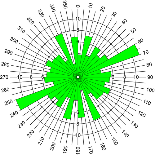
Figure 5.71 Rose diagram helps quantify the role of fractures.
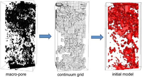
Figure 5.72 Transiting from macropore scale to an initial reservoir model, as experienced in Weyburn project of Canada.
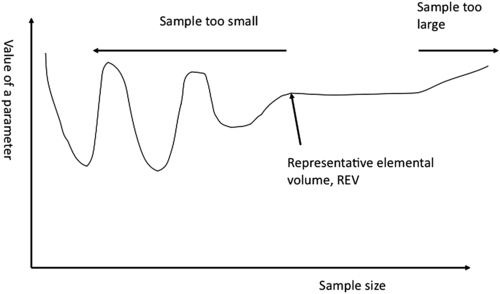
Figure 5.73 REV for a reservoir is much larger than the core samples collected.
5.8.1. Filtering Permeability Data
One of the most difficult problems in reservoir engineering is the fact that it is practically impossible to extract a sample that represents the reservoir. It is because the REV for petroleum reservoirs is much larger than the core size commonly encountered in a reservoir. Figure 5.73 highlights this difficulty. If the core size is below REV, all experiments conducted in it would have little relevance to the reservoir. This problem is further compounded in presence of fractures. The presence of fracture increases the size of REV and places a cored sample squarely in the oscillating region of Figure 5.73. In addition, coring in fractured formations is performed by avoiding the fractures as much as possible. This is because it is practically impossible to conduct fluid flow tests in a fractured core. For EOR design, this is of particular concern as the nature of fluid flow in a fractured formation is entirely different from that in a homogeneous system. Furthermore, flow that follows a certain regime (e.g., stable and stabilized) is likely to be different in presence of fractures. Because currently used instability number formulations do not use the presence of fractures (open or closed), it becomes even more difficult to predict the onset of fingering during an EOR process. However, fingering can lead to catastrophic failure of an EOR scheme.
In order to avoid this problem, filtering should be performed. Any such filter has to be custom designed for a specific field, if not specific well. For that, following data should be collected.
• Logs
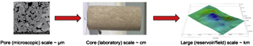
Picture 5.9 The idea is to transit from microscopic to reservoir scale, following the correct scaling laws.
• Maps
• Production data
• Well completion history
• Waterflood-injection history
• Any other data that may be available
At first, the full 3D schematic of the reservoir should be constructed. As depicted in Picture 5.9, the idea is to transit from microscopic scale to reservoir scale, which involves developing the scaling laws.
This schematic is not quantitatively accurate but represents overall trend. In order to decide on the schematic as well as the type of flow that is expected in the reservoir, geophysicists, geologists, and engineers must work together.
Based on that, one of the following averages should be used to construct the permeability (k) × net pay (h) correlation.
For parallel flow, arithmetic average should be used:
karith=∑ni=1kihi∑ni=1hi
![]()
For series flow, harmonic average should be used:
kharm=∑ni=1hi∑ni=1hi/ki
![]()
For flow without a particular pattern (random flow), geometric average should be used:
kgeom=n√k1k2k3…kn
![]()
At this point, well test results should be gathered and history of permeability variation with time should be collected. Quite often, well test permeability becomes a function of time. Such behavior gives out useful clues as to the nature of fluid flow in the reservoir. The knowledge of the operators, combined with the construction of geological history, and fluid flow behavior all contribute to determining the true nature of reservoir. For instance, consistent decline in reservoir permeability, as evidenced from well test data can occur because of fracture closure, asphaltene deposition, or formation of gas pockets in the neighborhood of the well. It is important to conduct laboratory tests in order to determine natural reaction to cores to stress. Figure 5.74 shows an example of such a test. In this laboratory simulation with artificially consolidated cores, the original stress corresponds to initial conditions of a reservoir, which is subject to little stress because of overall balance of forces. This is expected because over geological time, any reservoir reaches a state that can be termed steady state in conventional terminology. This stress is increased over time as more and more fluid is extracted from the reservoir. During this time period, original permeability can be reduced to less than 50% of the initial permeability. Many field history support this observation. For instance, in several of the giant oil field of Hassi Messaoud, Algeria, similar decline in well test permeability has been observed. The decline is steeper for more heterogeneous zones, the ones that have profuse fracturing.
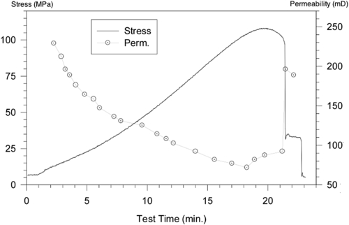
Figure 5.74 Laboratory test results under an overburden pressure of 50 MPa.
As can be seen in Figure 5.74, the core is crushed if the axial stress is very high (exceeding 100 MPa), resulting in sudden increase in permeability. Even then, however, original permeability is not restored. In theory, such occurrence of partial restoration of permeability can occur in the field. Several fields report such behavior. Almost all of these have fractures with intense network of secondary cementation.
In order to characterize a fractured formation, one has to know the following:
• The origin of formation
• The overall direction of flow
• Fracture distribution and frequency
One of the most useful tools of designing local filters is the compilation and plotting of hk from well tests and cores. In case of relatively homogeneous formation, the correlation between the two will follow the trend of a 45° straight line. Figure 5.74 demonstrates this point. On the other hand, if there are open fractures with significant aperture and length in the reservoir, the data points will fall over the straight line (meaning HKR is greater than unity, where HKR = ratio of hkwelltest/hkcore), the highest points representing maximum departure from the median line and highest frequency of open fractures. On the other hand, when points are located under the median straight line (meaning HKR less than unity), it signals the existence of secondary cementation that caused fractures to be plugged (Figure 5.75). For this case, the fraction of closed fractures over open fractures for various locations must be determined before a useful filter can be constructed.
This information is crucial to developing the filter. The filter uses the following data:
• frequency of open fractures
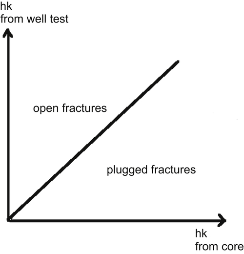
Figure 5.75 Determination of the nature of fractures from hk data.
• overall orientation of fractures
• overall orientation of sedimentation
5.8.2. Total Volume Estimate
Total volume estimate comes from the following sequential estimates.
1. Calculation based on geologic and seismic data;
2. Confirmation of hydrocarbon through well test (initial acidization and fracturing may be necessary);
3. The concept of net thickness does not apply;
4. Saturation cannot be estimated with logs in most cases;
5. Saturations must be confirmed with special core analysis;
6. End points are the only relevant points in a relative permeability curve;
7. Capillary pressure data is the basis for fine tuning total thickness, which is the determining factor for initial gas in place.
5.8.3. Estimates of Fracture Properties
TOC changes in shale formations influence Vp, Vs, density, and anisotropy and thus should be detected on the seismic response. To detect it, different workflows have been discussed by Chopra et al. (2012). Rickman et al. (2008) showed that brittleness of a rock formation can be estimated from the computed Poisson's ratio and Young's modulus well log curves. This suggests a workflow for estimating brittleness from 3D seismic data, by way of simultaneous prestack inversion that yields Ip, Is, Vp/Vs, Poisson's ratio, and in some cases meaningful estimates of density. Zones with high Young's modulus and low Poisson's ratio are those that would be brittle as well as have better reservoir quality (higher TOC, higher porosity). Such a workflow works well for good quality data and is shown in flow chart below.
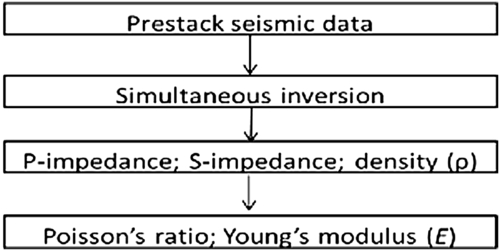
Natural fracture distribution map should be an indicator of how induced fracture will behave. Therefore, the data collected on natural fractures should be processed for designing an induced fracture.
Stress data collected during drilling as well as cuttings and well site logs should be all combined to develop enhanced understanding of reservoir fracture properties.
5.9. Special Considerations for Shale
Some of the considerations of reservoir characterization must be altered for shale due to unique features of shale gas. Picture 5.10 shows how induced fracture would propagate in shale. Scenarios 1, 2, and 3 represent theoretically likely directions of fracture propagation resulting from increasingly higher levels of fracture-inducing force. As force increases in relatively unfractured rock, fractures propagate perpendicular to the direction of maximum principal stress. When they encounter a rock layer boundary (which is naturally weaker), the energy forcing the fracture dissipates laterally, making it harder for a fracture to continue across boundaries. In more fractured rock (scenario 3a), even with the same pressures as seen in 3, preexisting fractures can cause energy forcing a fracture to dissipate in other directions. Because of the many boundaries between rock layers and preexisting fractures in scenario 3a, the fractures propagated are wider and shorter than they would normally be if the same rock was relatively unfractured.
Passey et al. (1990) proposed a technique for measuring TOC in shale gas formations. This technique is based on the porosity–resistivity overlay to locate hydrocarbon bearing shale pockets. Usually, the sonic log is used as the porosity indicator. In this technique, the transit time curve and the resistivity curves are scaled in such a way that the sonic curve lies on top of the resistivity curve over a large depth range, except for organic-rich intervals where they would show crossover between themselves.
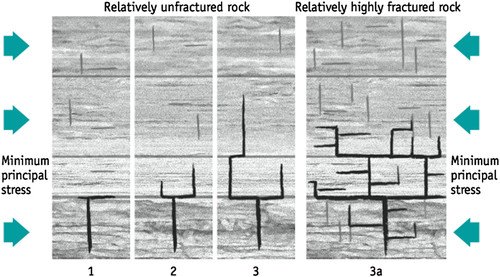
Picture 5.10 Different scenarios in fractured shale formation.
An integrated workflow in which well data as well as seismic data are used to characterize the hydrocarbon bearing shale can be developed as shown in the following workflow.
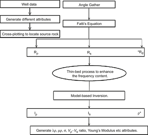
This compilation begins with the generation of different attributes from the well log curves. Then, using the cross-plots of these attributes one can identify the hydrocarbon bearing shale zones. Once this analysis is done at the well locations, seismic data analysis is picked up for computing appropriate attributes. Seismically, prestack data is essentially the starting point. After generating angle gathers from the conditioned offset gathers, Fatti's equation (Fatti et al., 1994) can be used to compute P-reflectivity, S-reflectivity, and density, which depends on the quality of input data as well as the presence of long offsets. Due to the band-limited nature of acquired seismic data, any attribute extracted from it will also be band-limited, and so will have a limited resolution. While shale formations may be thick, some high TOC shale units may be thin. So, it is desirable to enhance the resolution of the seismic data. An appropriate way of doing it is the thin-bed reflectivity inversion (Chopra et al., 2006; Puryear and Castagna, 2008). Following this process, the wavelet effect is removed from the data and the output of the inversion process can be viewed as spectrally broadened seismic data, retrieved in the form of broadband reflectivity data that can be filtered back to any bandwidth. This usually represents useful information for interpretation purposes. Thin-bed reflectivity serves to provide the reflection character that can be studied, by convolving the reflectivity with a wavelet of a known frequency band-pass. This not only provides an opportunity to study reflection character associated with features of interest, but also serves to confirm its close match with the original data. Further, the output of thin-bed inversion is considered as input for the model based inversion to compute P-impedance, S-impedance, and density. Once impedances are obtained, one can compute other relevant attributes, such as the λρ, μρ, and Vp/Vs. These are used to measure the pore space properties and get information about the rock skeleton. Young's modulus can be treated as brittleness indicators and Poisson's ratio as TOC indicator.
5.10. Special Considerations for Coalbed Methane
Methane within coalbeds is not structurally “trapped” by overlying geologic strata, as in the geologic environments typical of conventional gas deposits. Only about 5–9% of the CBM is present as “free” gas within the joints and cleats of coalbeds. Most of the CBM is contained within the coal itself (adsorbed to the sides of the small pores in the coal). Picture 5.11 shows a typical CBM reservoir, along with fracturing operations.
Before CBM production begins, groundwater and injected fracturing fluids are first pumped out (or “produced” in industry terminology) from the network of fractures in and around the coal zone. The fluids are pumped until the pressure declines to the point that methane begins to desorb from the coal. CBM production initially requires pumping and removing significant amounts of water to sufficiently reduce the hydrostatic pressure in the subsurface so that methane can desorb from the coal before methane extraction can begin. CBM is produced at close to atmospheric pressure. The proportion of water to methane pumped is initially high and declines with increasing CBM production (Figure 5.76). In contrast, in the production of conventional petroleum-based gas, the production of gas is initially high, and as gas production continues over time and the gas resources are progressively depleted, gas production decreases and the amount of water pumped increases.
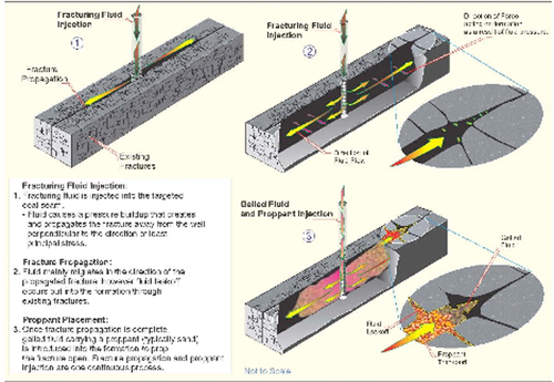
Picture 5.11 Schematic of a CBM with fracturing activities.
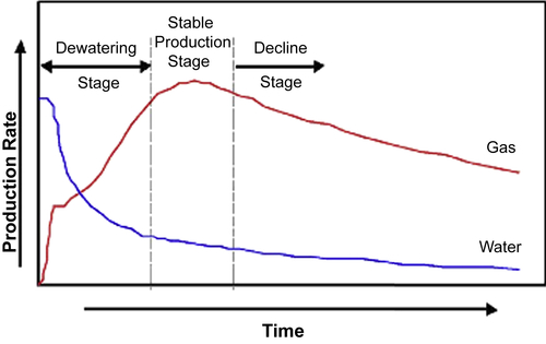
Figure 5.76 Production of water in CBM declines with time.
Almost every coalbed targeted for methane production must be hydraulically fractured to connect the production wellbore to the coalbed fracture network unless displacement or in situ combustion techniques are introduced. Many CBM wells are refractured at some time after the initial treatment in an effort to reconnect the wellbore to the production zones to overcome plugging or other well problems. Also, in response to site-specific coal geology and the economics of CBM production, where coal seams are thin and vertically separated by up to hundreds of feet of intervening rock, operators might design fracture treatments to enhance the vertical dimension and perform several fracture treatments within a single well to produce methane in an economically viable fashion.
..................Content has been hidden....................
You can't read the all page of ebook, please click here login for view all page.