
Chapter 3
Important Features of Unconventional Gas
Abstract
Unconventional gas reservoirs are loosely defined as those that cannot be produced with conventional techniques. It turns out that the volume of gas available increases exponentially as one moves from conventional gas to Coalbed methane, then to tight sand and shale gas, and then finally to gas hydrate deposits. For instance, gas hydrate volume is hundreds of times greater in methane volume than other sources of methane. At the same time, the quality as well as environmental integrity is also higher with more abundant gas resources. In this chapter, the most important features of gas with geological background are presented. This is followed with the process that is involved in forming natural gas through various physicochemical processes. At the end, it is demonstrated that unconventional gas is also the “cleanest” form of energy available today. This finding demystifies the global warming debate and puts all petroleum resources in its proper perspective.
Keywords
CBM; Gas hydrate; Global warming; Resource triangle; Shale gas; Tight gas3.1. Summary and Introduction
Unconventional gas reservoirs are loosely defined as those that cannot be produced with conventional techniques. It turns out that the volume of gas available increases exponentially as one moves from conventional gas to coalbed methane (CBM), then to tight sand and shale gas, and then finally to gas hydrate deposits. For instance, gas hydrate volume is hundreds of times greater in methane volume than other sources of methane. At the same time, the quality as well as environmental integrity is also higher with more abundant gas resources. In this chapter the most important features of gas are presented. They deal with both source and the process of gas formation. As such, geological background is presented. This is followed with the process that is involved in forming natural gas through various physicochemical processes. At the end, it is demonstrated that unconventional gas is also the “cleanest” form of energy available today. This finding demystifies the global warming debate and puts all petroleum resources in its proper perspective.
U.S. Bureau of Mines and U.S. Geological Survey (1980) produced the following figure (Figure 3.1) that shows the dynamic relationship between two most important factors, namely, economics and geology. The overall movement of petroleum resources is to the right as accumulations are discovered and upward as development and production ensue. The degree of uncertainty as to the existence of resources decreases to the right in the diagram. The degree of economic viability decreases downward and also implies a decreasing certainty of technologic recoverability. The two boundaries related to conventional– unconventional and recoverable–unrecoverable are flux due to changing economic viability over time, the role of sustainability, and social constraints. Significant changes in the cost/price relationship or fundamental changes in technologic capabilities can shift these boundaries, causing modifications in perceptions and the practical meaning of the definitions. Thus, uncertainties in economic and technologic conditions contribute to the substantial uncertainties in the resource assessment.
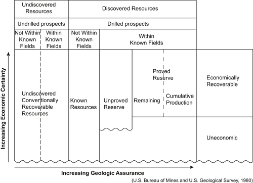
Figure 3.1 Interplay between economics and geological assurance.
As perceptive Lewis Weeks (1958), in considering this issue, wrote:
“While research adds to our proved reserves by developing new ways to find and produce oil, it is a field of activity whose advances are impossible to predict. This is because they depend to a large degree on such important, intangible human resources as initiative and ingenuity.”
“… man's mind is his most valuable asset— a ‘natural resource’ of unlimited potential— and the key to an abundant supply of fuel in the future.”
It is to be recognized that technological development is linked with economics; this aspect will be discussed later. In order to assure cohesion with existing literature, the following conventional definitions are introduced.
Conventionally recoverable: Producible by natural pressure, pumping, or secondary recovery methods such as gas or water injection.
Marginal probability of hydrocarbons: An estimate, expressed as a decimal fraction, of the chance that an oil or natural gas accumulation exists in the area under consideration. The area under consideration is typically a geologic entity, such as a pool, prospect, play, basin, or province; or a large geographic area such as a planning area or region. It is a matter of probability before drilling but it becomes a certainty for a drilled well but a matter of probability with greater certainty for other regions.
Resources: Concentrations in the earth's crust of naturally occurring liquid or gaseous hydrocarbons that can conceivably be discovered and recovered. Normal use encompasses both discovered and undiscovered resources.
Recoverable resources: The volume of hydrocarbons that is potentially recoverable, regardless of the size, accessibility, recovery technique, or economics of the postulated accumulations.
Conventionally recoverable resources: The volume of hydrocarbons that may be produced from a wellbore as a consequence of natural pressure, artificial lift, pressure maintenance (gas or water injection), or other secondary recovery methods. They do not include quantities of hydrocarbon resources that could be recovered by enhanced recovery techniques, gas in geopressured brines, natural gas hydrates (clathrates), or oil and gas that may be present in insufficient quantities or quality (low-permeability “tight” reservoirs) to be produced via conventional recovery techniques.
Remaining conventionally recoverable resources: The volume of conventionally recoverable resources that has not yet been produced and includes remaining proved reserves, unproved reserves, reserves appreciation, and undiscovered conventionally recoverable resources.
Economically recoverable resources: The volume of conventionally recoverable resources that is potentially recoverable at a profit after considering the costs of production and the product prices.
Undiscovered resources: Resources postulated, on the basis of geologic knowledge and theory, to exist outside of known fields or accumulations. Included also are resources from undiscovered pools within known fields to the extent that they occur within separate plays.
Undiscovered conventionally recoverable resources: Resources in undiscovered accumulations analogous to those in existing fields producible with current recovery technology and efficiency, but without any consideration of economic viability. These accumulations are of sufficient size and quality to be amenable to conventional primary and secondary recovery techniques. Undiscovered conventionally recoverable resources are primarily located outside of known fields.
Undiscovered economically recoverable resources: The portion of the undiscovered conventionally recoverable resources that is economically recoverable under imposed economic and technologic conditions.
Reserves: The quantities of hydrocarbon resources, which are anticipated to be recovered from known accumulations from a given date forward. All reserve estimates involve some degree of uncertainty.
Proved reserves: The quantities of hydrocarbons, which can be estimated with reasonable certainty to be commercially recoverable from known accumulations and under current economic conditions, operating methods, and government regulations. Current economic conditions include prices and costs prevailing at the time of the estimate. Estimates of proved reserves equal cumulative production plus remaining proved reserves and do not include reserves appreciation.
Remaining proved reserves: The quantities of proved reserves currently estimated to be recoverable. Estimates of remaining proved reserves equal proved reserves minus cumulative production.
Unproved reserves: Reserve estimates based on geologic and engineering information similar to that used in developing estimates of proved reserves, but technical, contractual, economic, or regulatory uncertainty precludes such reserves being classified as proved.
Reserves appreciation: The observed incremental increase through time in the estimates of reserves (proved and unproved (P and U)) of an oil and/or gas field. It is that part of the known resources over and above proved and unproved reserves that will be added to existing fields through extension, revision, improved recovery, and the addition of new reservoirs. Also referred to as reserves growth or field growth.
Total reserves: All hydrocarbon resources within known fields that can be profitably produced using current technology under existing economic conditions. Estimates of total reserves equal cumulative production plus remaining proved reserves plus unproved reserves plus reserves appreciation.
Total endowment: All conventionally recoverable hydrocarbon resources of an area. Estimates of total endowment equal undiscovered conventionally recoverable resources plus cumulative production plus remaining proved reserves plus unproved reserves plus reserves appreciation.
3.2. Overview of Unconventional Gas Reservoirs
Law and Curtis (2002) defined unconventional gas accumulations as follows:
“Conventional gas resources are buoyancy-driven deposits, occurring as discrete accumulations in structural and/or stratigraphic traps, whereas unconventional gas resources are generally not buoyancy- driven accumulations. They are regionally pervasive accumulations, most commonly independent of structural and stratigraphic traps.”
The regionally pervasive nature of unconventional oil and gas accumulations gives rise to very large resource volumes in most cases, and hence their significance is critical to assess. Natural distribution of energy sources is such that the volume of the reserve capacity increases as one moves away from conventional toward unconventional hydrocarbon resources.
Cander (2010) addressed the geological understanding of unconventional plays, noting:
“…the term ‘resource play’ implies to some that subsurface risks are either minimized or irreducible. As well, the term ‘unconventional gas’ connotes that little is to be gained from application of conventional principles of basin evolution and petroleum generation, migration, and entrapment. Under these circumstances, the value of regional geologic understanding of an entire basin prior to acreage capture can be overlooked.”
According to Cander (2010), it is important to understand a basin from basement to surface in assessing potential for unconventional hydrocarbon resources. This also bears relevance in terms of technologies required to unlock the gas.
3.2.1. The Resource Triangle
Figure 3.2 shows the schematic of the resource triangle concept that has been widely utilized for exploration as well as resource assessment of various commodities. Masters (1979) popularized the concept for gas reservoirs. This model has been applied in exploration and resource assessment for a number of different commodities and was popularized in the assessment of gas resources by Masters (1979). This triangle concept states that of the total resource base of a particular commodity, only a small proportion—near the apex of the triangle—is contained in high-quality reservoirs or deposits. Much greater resource volumes occur in poorer quality deposits, lower in the body of the triangle. For gas and oil, it is recognized that only a very small proportion of the resource has migrated into and can be produced from high-quality “conventional” reservoirs—those that the industry has been drilling throughout most of its history. Much larger hydrocarbon volumes occur in the “unconventional” reservoirs.
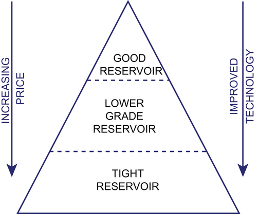
Figure 3.2 The resource triangle. After Masters, 1979.
It is generally understood that the relative magnitude of this growth is proportionally larger, the younger the field. This continuity is supported by the sustainability argument discussed in the previous chapter that showed biomass, which is the youngest form of carbon-energy source, is also the most abundant. However, when unconventional reserves are included a different factor enters the interplay. This is due to the types of reservoirs that enclose older form of energy but were previously excluded due to the lack of proper technology and/or favorable economic factors. Overall, the following factors play a role (Lore et al., 1999):
• areal extension of existing reservoirs,
• discovery of new reservoirs,
• increases in reserve estimates in existing reservoirs as production experience is gained,
• improved recovery technologies,
• increases in prices and/or reductions in costs, which reflect the influences of market economics and technology (revisions),
• field expansion via mergers with newer fields (extensions),
• systematic assessment bias toward conservatism, which typically exists in initial estimates of field sizes (revisions), and
• reporting practices with respect to proved reserves.
This triangle model also assumes that the technology has to be improved for accessing “lower quality” reservoirs. This assumption implies that the price of an energy source (or commodity) will increase. Even though this model is widely accepted in the petroleum industry, only recently Zatzman and Islam (2007) have challenged the validity of the model. Zatzman (2012a, 2012b) has subsequently demonstrated that these models are in fact misleading with worse implication for unconventional resources. This point should be discussed to some extent.
Traditionally, economic evaluations are based on cost per unit output, which is only suitable for determining short-term and tangible outlooks. A comprehensive economic evaluation of any system should include long-term considerations that are only captured through intangible elements. An evaluation that incorporates both the tangible and intangible elements may be considered truly comprehensive. An engineering decision support system that follows such an evaluation process will focus on the long term, even as it tests and selects ingenious solutions that are suitable for tangible and short-term applications. By focusing on the long term, the sustainability criterion is fulfilled, thereby eliminating long-term negative consequences of a short-term remedy. This chapter proposes a guideline of economic evaluation that will truly identify the best process among different processes for both short-term and long-term applications. The triangle model assumes that the technology developed strictly for short-term gains are indeed sustainable. This assumption is incorrect (Khan and Islam, 2012).
In most cases, the comparison of different processes is based on economic evaluation. In a conventional economic analysis, there is no room for distinguishing between an energy source that is nonrenewable and one that is renewable. In the information age, it has become clear that such a “fit for all” analysis technique is not appropriate for meeting the energy needs of the future (Zatzman and Islam, 2007). In the information age, it has become both necessary and possible to custom design a specific engineering application in order to ensure long-term sustainability. One can no longer count on the future in order to ensure that the short-term needs are fulfilled. Because of the sustainability crisis, conventional economics and accounting theories have lost their effectiveness. For instance, according to the supply-and-demand theory, the cost of products from limited resources will increase continuously with the increase of demand and depletion of the resources. This scenario holds the most severe consequences for any resource that is the driving force of civilization and is very limited in supply. With this mode, if current practices of energy production and utilization continue, there will be a huge shortage of energy in the near future. This is evident from the increase in gas prices within the last two decades, the recent tripling of oil prices that sparked worldwide financial crisis, and the most recent sharp drop in oil prices that made the financial crisis worse. Yet, the real value of crude oil did not change, just like the real value of soil or any other natural commodity. This is the reason Zatzman and Islam (2007) characterized this economic system as being based on perception and not knowledge.
The conventional economic theories can be directly linked to disinformation regarding the intangible–tangible nexus. The theories of modern economics taught today, all start from something called “the theory of marginal utility.” The English economics writer William Stanley Jevons (1870) first developed this theory in the 1870s, and it was furthered in the works of Carl Menger (1871), Leon Walras (1874), and Alfred Marshall (1890). Its underlying thesis, which became the basis of an elaborate theory known as neoclassical economics, is that endogenous “choices” about price operate entirely according to personal choice or desire for access to, and use of, some good or service, with the last unit of demand determining the price “at the margin.” All of this takes place without reference to any exogenous conditions such as the monopolized character of production, the cartelized character of international trade, or the role of imperial dictates, rivalries, and/or wars in suppressing or further distorting the operation of supply and demand. Consumption takes place without reference to how commodities were produced in the first place. How, indeed, could that which has not yet been produced supposedly be distributed and consumed? “At the margin,” reply the neoclassical economists. But one only has to ask the question, “whence the originating intention to consume or to produce?”
The specific role asserted for the theory of marginal utility in this arrangement reduces the domain of concern for “the margin,” so as to simplify handling the relevant variables. However, it is precisely in this process that the counterfeiting job is carried out, as all exogenous conditions beyond “the margin” are simply removed from the domain of consideration, including any condition (such as intention) that may play some role in defining the boundary of, and/or the conditions at, “the margin.”
The mathematical assumptions fundamental to the basic theory of marginal utility are another source of serious misdirection. Here, the still unaddressed question of intention becomes layered in further opacity. In order to model the individual's “choice” behaviors in economic reality, an untestable assumption that is completely subjective is used to measure what happens on a societal scale. That untestable assumption asserts that individuals' behaviors consist of maximizing personal pleasure and minimizing personal pain. This assumption is untestable because it assumes that society is composed of the individual multiplied uniformly and homogeneously over and over, or, in other words, that the individual exists, but society as a real category in its own right does not exist when it comes to economic analysis or decisions. To assert the existence of each would be true, but to hitch one (society) as subordinate to and derivative of the other (the individual) is false. In addition to this fundamental difficulty, this procedure also transfers the short-term perspective of the individual to society as a whole. However, since the death of any individual or individuals obviously cancels their personal term without shortening the term of society's existence, such a procedure is inherently and patently absurd.
Jevons, in particular, declared economic behavior to be nothing more or less than the materialization in social form of this allegedly universal and thoroughly selfish principle. What the worker does to avoid starvation is, thereby, equated with what the business owner does to get another few pennies of profit out of the powerless public. Jevons even suggested a mathematical model that justified his standpoint, arguing that the discrete choices of millions of economic actors may be approximated meaningfully or usefully by continuous-type mathematical functions. He combined this with the notion of processes that would eventually reach steady-state conditions, adapting to economics a mode of analysis that researchers in thermodynamics had pioneered widely by the middle third of the nineteenth century.
If the spurious assumption is removed, a new picture emerges from Figure 3.2. For instance, using truly sustainable technologies will make the downward arrows reversed. Indeed, Islam et al. (2010; 2012) and Khan and Islam (2012) have demonstrated that proper selection of technologies can align efficiency with sustainability, i.e., environmental integrity and economic benefits increase as one applies a sustainable technology to vaster resources. In this process, the qualities of gas, including its heating value and environmental integrity, are improved. Figure 3.3 shows this paradigm shift in unconventional gas.
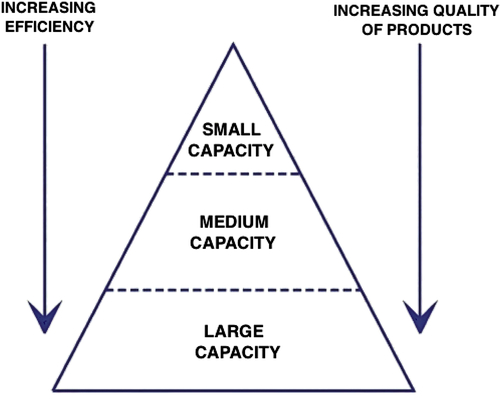
Figure 3.3 Paradigm shift in unconventional gas development.
In the incubation era of unconventional gas (2000–2008), the industry saw large gas price increases and tremendous advances in drilling and completions practices, such as extended-reach horizontal wells and multiple staged hydraulic fracture (“fracking”) stimulations. Unconventional gas production thus increased dramatically in the United States and to a lesser extent in Canada. Since 2008, however, world economic issues and the glut of new gas production on the North American market have depressed gas prices in North America. Industry is now turning more attention to unconventional plays that can produce liquid hydrocarbon resources from the lower part of the resource triangle. Such measures are not necessary if custom designed techniques are used rather than using blanket technologies for all resources. For instance, gas hydrate does not require any gas processing and burns easily. In addition, it is as abundant at the earth surface as tar sand. Why should this process be more expensive than natural gas that is produced from 10,000 ft below surface and contain high amount of toxic components?
By convention, several types of gas reservoirs are recognized, that are listed below:
• Coalbeds, hosting CBM, also known as coal seam gas;
• Tight reservoirs, both clastics and carbonates;
• shale reservoirs; and
• gas hydrates.
Shallow biogenic gas reservoirs have been considered by some as a distinct unconventional gas resource type (e.g., Shurr and Ridgley, 2002), but are now generally included with shale gas and tight gas resources.
3.3. Special Features of Unconventional Gas Reservoirs
The most commonly considered unconventional gas is shale gas, whereas the least heard unconventional resource is gas hydrate. Following is a brief description of these reservoirs.
3.3.1. Coalbed Methane
CBM is, as the name implies, a natural gas hosted in seams or beds of coal. Bustin and Clarkson (1998) described it as:
“Coalbed methane, unlike conventional gas resources, is unique in that gas is retained in a number of ways including: (1) adsorbed molecules within micropores (<2 nm in diameter); (2) trapped gas within matrix porosity; (3) free gas (gas in excess of that which can be adsorbed) in cleats and fractures; and (4) as a solute in ground water within coal fractures.”
Coalbeds are generally self-sourcing reservoirs—they contain gas evolved either biogenically or thermogenically from organic material within the coals themselves. In their original form, this gas contains all vital components of life form, such as, oxygen, nitrogen, water vapor, carbon dioxide, carbon monoxide, methane, ozone, nitrogen dioxide, nitric acid, ammonia and ammonium ions, nitrous oxide, sulfur dioxide, hydrogen sulfide, carbonyl sulfide, dimethyl sulfide, and a complex array of nonmethane hydrocarbons. It is interesting to note that only nitrogen and oxygen are not “greenhouse gases.” These biogenic gases are not accounted for global warming vulnerability when emitted from biomass. However, they are considered to be the primary reason for global warming when emitted through ‘petroleum activities’. CBM is distinct from a typical sandstone or other conventional gas reservoir, as the methane is stored within the coal by a process called absorption and adsorption. The methane is in a near-liquid state, lining the inside of pores within the coal (called the matrix). The open fractures in the coal (called the cleats) can also contain free gas or can be saturated with water.
Absorption refers to the process by which one substance, such as a solid or liquid, takes up another substance, such as a liquid or gas, through minute pores or spaces between its molecules. The absorption capacity of the absorber depends on the equilibrium concentrations between gaseous phase and the liquid phase. For diluted concentrations in many gases and in a wide interval of concentrations, the equilibrium relation is given by Henry's Law, which quantifies the gas absorption capacity in the fluid (Cengel and Boles, 2008). The most effective gas absorbing unit would ensure complete contact between the gas and the solvent, in such a way that diffusion occurs at the interphase. This is the case with CBM. For instance, with water, methane absorption efficiency is around 97%. It also simultaneously removes H2S when H2S is less than 300 cm3 and is adjustable to changing pressure or temperature.
In addition, adsorption also plays a big role in CBM. Adsorption refers to the process by which molecules of a substance, such as a gas or a liquid, collect on the surface of a solid. It differs from absorption, in which a fluid permeates or is dissolved by a liquid or solid (Tondeur and Teng, 2008). This process can be physical (reversible) or chemical (irreversible). In physical adsorption processes, gas molecules adhere to the surface of the solid adsorbent as a result of the molecule's attraction force (Van der Walls Forces). Chemical adsorption involves a chemical reaction. Coalbed is known to be the best of adsorbers. For instance, coalbed acts as a highly efficient methane adsorber (95–98% CH4). It is also excellent for capturing H2S at relatively low energy. The microstructure of coalbed is such that it acts as a natural filter. It has a high surface area ranging from 0.68 m2/g to 9.7 m2/g.
Furthermore, condensation plays a role in CBM. It is the process of converting a gas into a liquid by reducing temperature and/or increasing pressure. Condensation occurs when partial pressure of the substance in the gas is lower than the vapor pressure of the pure substance at a given temperature. As a coalbed is exposed to high pressure, condensation leads to compaction of the gas resource, making CBM to be commercially available within coalbed.
Finally, natural membrane separation plays a role in purifying methane. CBM as well as water films serve as a selective barrier between two phases and remain impermeable to specific particles, molecules, or substances when exposed to the action of a driving force. The driving force is the pressure difference between both sides of the membrane. Gas permeability through a membrane is a function of the solubility and diffusivity of the gas into the material of the membrane. Membranes are expensive and their separation efficiencies are low (Ramirez, 2007).
This gas is distinctly different from gas from other sources. The term refers to methane adsorbed into the solid matrix of the coal. It is called “sweet gas” because of its lack of hydrogen sulfide. The presence of this gas is well known from its occurrence in underground coal mining, where it presents a serious safety risk. CBM is distinct from a typical sandstone or other conventional gas reservoir, as the methane is stored within the coal by a process called adsorption. The methane is in a near-liquid state, lining the inside of pores within the coal (called the matrix). The open fractures in the coal (called the cleats) can also contain free gas or can be saturated with water.
Most facies models for coal-bearing strata show peat accumulating close to active clastic depositional environments, such as floodplains of meandering rivers, coastal mires, behind beach barriers or in interdistributary bays of deltas. In this, muds and slits are introduced during frequent floods, storm surges, or high tides (McCabe, 1988). Thick, low ash peat accumulations are most commonly formed in areas that were removed from active clastic deposition for long periods of time. Coal seams have complex internal stratigraphies that lead to considerable variation in plant types; early alteration of organic material and climate changes are important factors during peat accumulation. Variations in vertical profile of coal seams are observation based on maceral distribution and palynological studies (Hacquetard and Donaldson, 1969). Although some coals and adjacent clastics may have been deposited simultaneously, most common cases show that the contact between the two lighologies represents a considerable time gap in deposition. Peats commonly overlie much older sediments representing a 100,000 year of more hiatus (Figure 3.4).
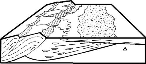
Figure 3.4 Schematic showing tectonic controls of coal deposition during the early tertiary in the Alberta basin. Richardson et al., 1988.
In some cases, thick accumulations of peat sit directly on Pleistocene beach ridges in areas unaffected by storms and tidal surges. These mires develop extensive, low ash peats unhindered by clastic sources. Mires can be classified into three types: raised, low-lying, and floating. Low-lying mires form in areas of poor drainage. Floating mires develop over lakes until the lake infills with sediment or peat and can later develop into larger low-lying mires. If climate conditions permit, a raised mire can develop. Raised mires occur in areas where annual precipitation is greater than annual evaporation, which occur in maritime environments. There has to be a balance between preservation and deterioration of organic matters. For instance, most tropical rainforests are not sites of peat accumulation as the organic matter deteriorates rapidly.
The alluvial plain environment is characterized by widespread mires and very long gradients. For many cases, associated sediments are predominantly fluvial in origin. A moderately low ash content and laterally persistent and relatively think nature of many of these coal seams would indicate the development of widespread mires isolated from clastic deposition for long periods of time.
The key parameters that control gas resource quantities and producibility are
• thermal maturity—sorption capacity generally increases with maturity;
• maceral composition—sorption capacity increases with vitrinite content, and decreases with inertite content and mineral matter;
• reservoir pressure—generally increases with depth;
• coal thickness;
• fracture (cleat) density;
• permeability, which is a function of burial history, burial depth, and in situ stresses; and
• hydrologic setting, which dictates how much water is present in coal seams (Ayers, 2002).
CBM is formed in confined coalbed aquifers through complex biogeophysical processes and remains trapped by water pressure. Coalbed natural gas-produced water can have high concentrations of soluble salts (Rice et al., 2000). The above mentioned factors play significant roles in forming and transporting of CBM. Figure 3.5 shows how the process acts like a water filter. CBM has a biogenic root. The biogenic gas falls into two distinct systems that have different attributes. Early-generation systems have blanketlike geometries, and gas generation begins soon after deposition of the source rock. Late-generation systems have ringlike geometries, and long time intervals separate deposition of reservoir and source rocks from gas generation. For both types of systems, the gas is dominantly methane and is associated with a water system. In certain cases, biogenic gas will be transformed through thermogenic processes. When these fine-grained sediments are buried by deposition of later, overlying sediments, the increasing heat and pressure resulting from burial turns the soft sediments into hard rock strata. If further burial ensues, then temperatures continue to increase. When temperatures of the organic-rich matrix exceed 120 °C the organic remains begin to be “cooked” and more natural gas is formed.
Figure 3.6 shows coalbed matrix that embeds gas surrounding the coal bound by water and rock. Note that the light blue represents gas that is held in contact with the coal through high water pressure. Water remains in cleats and fractures. This schematic explains how CBM is one of the cleanest site of methane. Both coal and water are most potent contaminant separating agents. Both gaseous and liquid contaminants can be separated in this process.
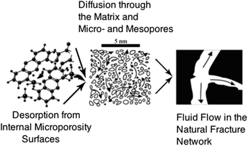
Figure 3.5 Microscopic process of CBM transport.
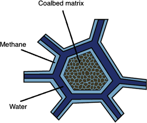
Figure 3.6 Schematic of CBM surrounded by water.
Cleats are fractures that usually occur in two sets that are, in most instances, mutually perpendicular and also perpendicular to bedding. Although pre-1990 geologic literature and current mining usage distinguishes these sets on the basis of factors such as “prominence” that are difficult to quantify, abutting relations between cleats generally show that one set predates the other. Picture 3.1 shows the existence of cleats in Alberta outcrops. Through-going cleats formed first and are referred to as face cleats; cleats that end at intersections with through-going cleats formed later and are called butt cleats (Laubach and Tremain, 1991; Kulander and Dean, 1993). These fracture sets, and partings along bedding planes, impart a blocky character to coal.
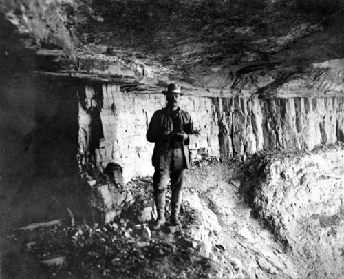
Picture 3.1 Coal outcrop from Utah. USGS file photo.
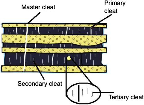
Figure 3.7 The existence of various cleats within coalbed.
Coal cleat is important in enhancing CBM potential, as it is these interconnected fracture networks (permeability) that allow fluids (water and gas) to move through the coals and into a wellbore for production. The widths or openings of cleats are generally wider near the surface, but with increasing depth the weight of the overlying rock compresses, or closes the cleats, reducing their width and connectivity (reducing reservoir permeability). Cleats may be enhanced in areas of faulting, fracturing or where coal seams may be draped over sandstone channels. CBM companies are always looking for areas of enhanced permeability to improve their exploration success potential. Figure 3.7 shows the existence master cleat, primary, secondary, and tertiary cleat within the cola matrix.
3.3.1.1. Coal Rank, Depth of Cover, and CBM Potential
One of the most important features of coalbed is that as the depth increases the gas content is increased whereas the fracture openings are restricted. This leads to the existence of optima in terms of depth of a coalbed.
3.3.2. Tight Gas
Unconventional tight oil and gas resources are generally found in basin-centered systems, defined by Law (2002) as:
“…regionally pervasive accumulations that are (hydrocarbon) saturated, abnormally pressured, commonly lack a downdip water contact, and have low-permeability reservoirs.”
In general, the term “hydrocarbon saturated” refers to oil or gas that occupies most of the reservoir pore volume (generally >75%), and that one or both of these phases flow from the formation; however, there is almost always some residual water saturation. “Abnormal pressures” indicate that the hydrocarbon phase is not connected to a regional aquifer—pressures may be relatively high or low compared to a normal hydrostatic gradient (and may be both in different regions of a given basin). “Low permeability” is a term that has been used in a variety of ways, but the most commonly accepted definition is that “tight” gas reservoirs have maximum in situ permeabilities of <0.1 mD, with the implication that natural or artificial fracture stimulation is required for economic production. This definition of Law (2002) excludes many reservoirs that have high water content. Also, the definition in terms of low permeability has been accepted worldwide, while keeping open the arbitrary nature of the cutoff point of 0.1 mD. Often, this “low permeability” is linked with need to fracture a formation in order to make the gas flow economically. Others have defined tight gas reservoirs as being the ones that cannot be produced at economic flow rates or recover economic volumes of gas unless the well is stimulated by a large hydraulic fracture treatment and/or produced using horizontal wellbores (Holditch, 2007, 2006). This definition is also applied to CBM, shale gas, and tight carbonate reservoirs. There is no typical tight gas reservoir, it can be: deep or shallow, high pressure or low pressure, high temperature or low temperature, homogeneous or naturally fractured (heterogeneous), single or multilayered, high transient decline rates, comingled production; require fracturing jobs and/or horizontal well. In other words, tight gas is gas that is “trapped‟ in a very tight formation underground, stored within low-porosity and low-permeability rock formations. In general, it is commonly understood, there are only two options for recovering this gas. They are fracturing and drilling horizontal wells.
Source rocks for basin-centered accumulations are commonly found interbedded within or downdip of the tight reservoir section. Hydrocarbons thus charge the system directly, without migration through and exposure to regional aquifer systems (Welte et al., 1984; Law, 2002). Strong aquitards, such as thick, continuous marine shales, also assist in isolating basin-centered accumulations from contact with regional aquifers.
A play is defined as a group of reservoirs genetically related by depositional origin, structural style or trap type, and nature of source rocks or seals (White and Gehman, 1979; White, 1980). A typical tight play consists of grouped reservoirs (termed pools or accumulations) within individual fields that produce from the same chronozone and depositional sequence. These pools often vertically stacked within fields (Figure 3.8).
A key feature in the current exploitation of most basin-centered tight gas systems is the presence of a relatively thick (tens to hundreds of meters) column of hydrocarbon-saturated rock. Gas resources in place per unit area (often expressed as Bcf per section—billion cubic feet per one-mile-square section of land) are thus high—up to tens of Bcf per section. Alternatively, a tight gas or oil reservoir may be thinner, but very laterally extensive—allowing highly-repeatable drilling strategies over large areas. Using appropriate drilling and completions strategies, each well can access an economic reserves volume, despite low formation permeabilities.
A typical depositional model is shown in Figure 3.9. This particular example has three depositional styles (retrogradational, aggradational, and progradational) and one depositonal facies (fan). The retrogradational style, characterized by thick shale sections and thin sandstone beds, represents major or widespread transgressive events. The lower part of the retrogradational section commonly contains thin sandstone units that are products of reworking of the top of the underlying shallow-water sandstones. Within the retrogradational package are thinner packages of sandstone that typically comprise upward-coarsening progradational parasequences. When stacked, the thin progradational parasequences form a back-stepping architecture, reflecting the increasing amount of accommodation space and the retreat of depositional environments during relative sea-level rise.
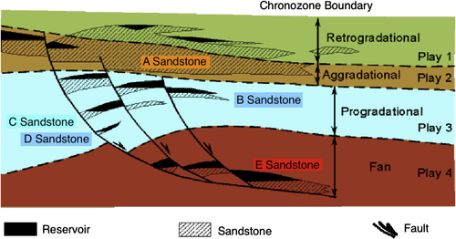
Figure 3.8 Stacked pools. From Lore et al., 1999.
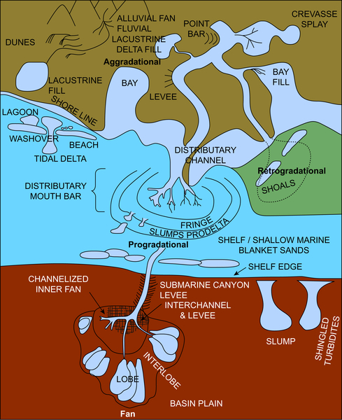
Figure 3.9 Model for deltaic deposition. From Lore et al., 1999.
The aggradational style comprises thick sandstone beds separated by thin shale units. Depositional environments represented by aggradational sediments include fluvial–streamplain, bay–lagoon, barrier island, coastal strandplain, and marine shelf (Morton et al., 1988). Fluvial and strandplain depositional environments dominate the aggradational depositional style.
The progradational style is characterized by deeper water shale at the base, along with thin sandstone units that grade upward into dominantly shallow marine deltaic and shoreline sandstones that are topped by thin shale interbeds. A broad spectrum of paralic depositional environments, including deltaic, shoreline, strandplain, barrier bar, shelf, and coastal plain, are subsumed under the progradational style. Deltaic depositional environments are dominant. Progradational architecture is constructed of thinner packages of dominantly progradational parasequence sets. Minor or local retrogradational events are typically interspersed within the overall progradational style.
The fan facies is a sandstone-rich, deepwater environment, characterized by a variable pattern of sandstone-body thickness (including thick to thin and blocky to upward-fining sandstones), sharp-based channel-fill sandstones, and serrated, thin to thick sandstones interbedded with thick shale units. Fan environments are characteristically overlain by hundreds of feet of deepwater shale.
The continental environment has the following systems:
Eolian systems
Lacustrine systems
Fluvial systems
Terrigenous fan (alluvial fan and fan-deltaic systems)
The shoreline environment has the following systems:
Delta systems
Barrier-strandplain systems
Lagoon, bay, estuarine, and tidal-flat systems
Marine environments has the following systems:
Continental and intracratonic shelf systems
Continental and intracratonic slope and basinal systems
These features show up in spontaneous potential data, as shown in Figure 3.10. This figure also shows characteristic features of each layer.
For Gulf of Mexico, Lore et al. (2001) described some of the important features of various styles.
The main characteristic of retrogradational deposit is the existence of upward-coarsening and upward fining of thin sandstone and upward-thinning packages of sandstone. The depositional environments are back-stepping assemblage of shoreline, deltaic, and nearshore environments that culminate in open-shelf mud-rich settings. They are typically capped by a flooding surface coincident with a chronozone boundary.
The aggradational style shows thick, blocky stacked sandstone. The environment shows the existence of vertically stacked upper alluvial plain, valley-fill, fluvial crannel, overbank, upper-delta plain, sand-rich deposits.
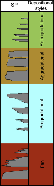
Figure 3.10 Electric characteristics of various depositional styles. From Lore et al., 1999.
The progradational layer is characterized by thin to thick, upward-coarsening sandstone and sandstone packages. The depositional environment is regressive assemblage of environments grading from relatively deepwater mud-rich distal deltaic environments that grade upward to relatively shallow-water paralic and sand-rich deltaic and shoreline environments. Typical overlying a chronozone boundary in proxima position are fan systems in distal position.
The fan style is characterized with serrated, thin to thick sandstone packages, thick shale at top, upward fining, blocky at base with singular or stacked settings. The environment has upper-slop to abyssal-plain environment comprising channel fill, levees, and overbank sands deposited in a relatively sand-rich deepwater environment (Table 3.1).
The classic example of a basin-centered gas system is the San Juan Basin of the Western United States. Masters (1979) demonstrated the widespread occurrence of gas in low-permeability Cretaceous reservoirs in the center of the basin, downdip from regional aquifers around the basin margins (Figure 3.11). Hayes (2005) reviewed some of the key advances throughout this time in recognizing the importance and characteristics of tight gas resources.
Table 3.1
Summarizes the Clastic Sedimentary Environment
| Environment | Agent of transportation deposition | Sediments |
| Alluvial | Rivers | Sand, gravel, mud |
| Lake | Lake currents, waves | Sand, mud |
| Desert | Wind | Sand, dust |
| Glacial | Ice | Sand, gravel, mud |
| Delta | River, waves, tides | Sand, mud |
| Beach | Waves, tides | Sand, gravel |
| Shallow shelf | Waves, tides | Sand, mud |
| Deep sea | Ocean currents, settling | Sand, mud |
Law (2002) formalized the definition of basin-centered gas, and tabulated numerous examples of basin-centered gas accumulations in the United States and internationally. Moslow (2005) summarized characteristics of Western U.S. Rocky Mountain tight gas reservoirs as follows:
• Thick (tens to hundreds of meters), laterally extensive sandstones;
• Low porosities (8–12%) and permeabilities (<0.1 mD);
• Generally high sand/shale ratios;
• Extensive natural fracturing, arising from the complex tectonic history of most U.S. Rocky Mountain basins; and
• Abnormal reservoir pressures (predominantly overpressured).
Masters (1979, 1984) proposed a somewhat different model for regionally extensive low-permeability gas reservoirs along the western flank of the Western Canada Sedimentary Basin within a basin-centered gas system, calling it the Deep Basin. This model is shown in Figure 3.12. The system is sourced from coaly strata interbedded within the tight gas section and from regional marine source rocks, occurring downsection and downdip in the gas window. Thick marine shales cap Deep Basin reservoirs and isolate them from shallow aquifers and meteoric waters. While many geologists were initially reluctant to accept the Deep Basin concept, the success of Canadian Hunter Exploration in discovering widespread subnormally pressured gas pools, not connected to updip regional aquifers, provided evidence of the existence of Deep Basin. However, these early discoveries tapped into “stratigraphic sweet spots” within the Deep Basin—relatively small bodies of coarse clastic strata featuring conventional reservoir quality—such as shoreline-deposited conglomerates in the Cadotte and Falher members (Masters, 1984). In this, enormous amount of gas and liquid resources in the truly low-permeability rocks were not being accessed.
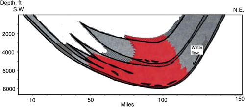
Figure 3.11 Schematic cross section of San Juan Basin, showing basin-centered gas system (in deep grey) From Masters (1979).
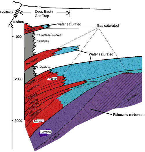
Figure 3.12 Schematic cross section of Western Canada Deep Basin, showing continuous gas-saturated reservoirs downdip from regional aquifers. (Redrawn from Hayes and Archibald, 2012).
Deep Basin tight gas reservoirs host huge gas resources in Alberta and British Columbia. Initial estimates show the following numbers:
• Gas in place, Alberta Deep Basin, Townships 45–75: 430 Tcf (Hayes et al., 2009);
• Gas in place, northeast British Colombian Deep Basin: 111–260 Tcf (Hayes, 2003; Hayes and Hayes, 2004); and
• Gas in place, Montney Deep Basin: corporate report and analyst figures ranging from tens to hundreds of Bcf per section, for a total play potential of hundreds of Tcf.
Hayes (2010), in an initial scoping assessment of tight gas potential in the Northwest Territories, concluded that tight gas potential may exist in specific Cambrian depocenters in the Colville Hills area, in the Devonian Imperial Formation of Peel Plain, and in Cretaceous, Triassic, and Devonian Jean Marie tight gas plays mapped northward from Alberta and British Colombia into southern Northwest Territories. Elsewhere in Canada, tight gas potential has generally not been assessed systematically—in part because it is difficult to establish the existence of all the components of a tight gas petroleum system where drilling and testing are sparse. Documentation of complete petroleum systems and conventional petroleum plays in Paleozoic basins of eastern Canada by Lavoie et al. (2009) and Dietrich et al. (2011) suggests that numerous tight gas and oil plays may exist there.
3.3.3. Shale Gas Reservoirs
Shale gas been in the core of recent domestic gas production revolution in the United States. It is expected that this superflux of gas would reverse the expectation that the United States remain a substantial gas importer, and has contributed to reduced gas prices, and enhanced industrial competitiveness. Overall, it is predicted that shale gas would exhibit the fastest growth in production within the United States, making an example for the rest of the world to follow.
Curtis (2002) defined shale reservoirs as:
fine-grained, clay- and organic carbon-rich rocks, [which] are both gas source and reservoir rock components of the petroleum system…Gas is of thermogenic or biogenic origin and stored as sorbed hydrocarbons, as free gas in fracture and intergranular porosity, and as gas dissolved in kerogen and bitumen.
Similar to most nomenclature, the term “shale” is not scientific because gas can be present in many other forms of rocks that have similar properties. This was pointed out by Rokosh et al. (2009) that stated: gas can be present “not only in shale, but also a wide spectrum of lithology and texture from mudstone to siltstone and fine-grained sandstone, any of which may be of siliceous or carbonate composition.”
Hamblin (2006) also noted the compositional variability of “gas shales,” and defined them more broadly, in terms of unconventional accumulations:
These are unconventional, basin-centered, self-sourced, continuous-type gas accumulations where the total gas charge is represented by the sum of free gas and adsorbed gas…In effect, these shale gas plays represent discrete, self-enclosed petroleum systems which do not rely on hydrocarbon expulsion/migration/trapping because the premise is that the hydrocarbon stays in the original source rock; if they were well-connected to conventional plays, then they wouldn't provide a new play at all.
Practically all caprocks will have similar properties. The common practice is to use certain cutoff point in terms of porosity or saturation or permeability in conventional reservoir analysis. However, this practice loses meaning when it comes to unconventional gas and oil. Vast majority of caprock will have certain amount of gas that can be considered part of the unconventional reserve.
Shale gas reservoirs have the following features:
• Rock volume—the entire thickness and areal extent of the shale has the potential of producing gas as long as special techniques are used;
• Total organic carbon content will be mainly distributed as adsorbed to the rock surface and along the fractures and fissures;
• Mature organic materials that are closest to the source rock;
• Mineralogical composition of the shale and related rocks is such that the rock is brittle;
• Natural fractures and fissures are present; and
• High water saturation.
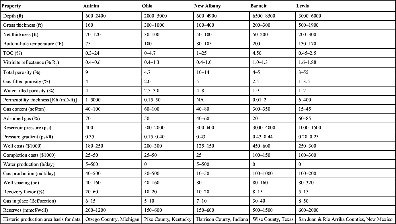
The above features are all relevant and exploitable as long as the right technology is employed. To date, horizontal wells and fracking remain the only two techniques vastly employed in the petroleum engineering industry. However, there are no optimal values for these parameters, but the characteristics of each shale reservoir dictate the most appropriate drilling, completion, and production strategies. As each new shale play unfolds, operators must undertake a period of experimentation in order to refine these strategies. Several workers, such as Curtis (2002), have tabulated selected parameters for various shale plays (Table 3.2).
Table 3.2
Geological, Geochemical, and Reservoir Parameters for Five Shale Gas Systems in the United States
| Property | Antrim | Ohio | New Albany | Barnett | Lewis |
| Depth (ft) | 600–2400 | 2000–5000 | 600–4900 | 6500–8500 | 3000–6000 |
| Gross thickness (ft) | 160 | 300–1000 | 100–400 | 200–300 | 500–1900 |
| Net thickness (ft) | 70–120 | 30–100 | 50–100 | 50–200 | 200–300 |
| Bottom-hole temperature (°F) | 75 | 100 | 80–105 | 200 | 130–170 |
| TOC (%) | 0.3–24 | 0–4.7 | 1–25 | 4.50 | 0.45–2.5 |
| Vitrinite reflectance (% R0) | 0.4–0.6 | 0.4–1.3 | 0.4–1.0 | 1.0–1.3 | 1.6–1.88 |
| Total porosity (%) | 9 | 4.7 | 10–14 | 4–5 | 3–55 |
| Gas-filled porosity (%) | 4 | 2.0 | 5 | 2.5 | 1–3.5 |
| Water-filled porosity (%) | 4 | 2.5–3.0 | 4–8 | 1.9 | 1–2 |
| Permeability thickness [Kh (mD-ft)] | 1–5000 | 0.15–50 | NA | 0.01–2 | 6–400 |
| Gas content (scf/ton) | 40–100 | 60–100 | 40–80 | 300–350 | 15–45 |
| Adsorbed gas (%) | 70 | 50 | 40–60 | 20 | 60–85 |
| Reservoir pressure (psi) | 400 | 500–2000 | 300–600 | 3000–4000 | 1000–1500 |
| Pressure gradient (psi/ft) | 0.35 | 0.15–0.40 | 0.43 | 0.43–0.44 | 0.20–0.25 |
| Well costs ($1000) | 180–250 | 200–300 | 125–150 | 450–600 | 250–300 |
| Completion costs ($1000) | 25–50 | 25–50 | 25 | 100–150 | 100–300 |
| Water production (b/day) | 5–500 | 0 | 5–500 | 0 | 0 |
| Gas production (mdt/day) | 40–500 | 30–500 | 10–50 | 100–1000 | 100–200 |
| Well spacing (ac) | 40–160 | 40–160 | 80 | 80–160 | 80–320 |
| Recovery factor (%) | 20–60 | 10–20 | 10–20 | 8–15 | 5–15 |
| Gas in place (Bcf/section) | 6–15 | 5–10 | 7–10 | 30–40 | 8–50 |
| Reserves (mmcf/well) | 200–1200 | 150–600 | 150–600 | 500–1500 | 600–2000 |
| Historic production area basis for data | Otsego Country, Michigan | Pike County, Kentucky | Harrison County, Indiana | Wise County, Texas | San Juan & Rio Arriba Counties, New Mexico |
ac = acre
From Curtis, 2002.
Historically, shale gas development in the United States has been synonymous Devonian shales. As early as 1821, these formations have been set in production in the Appalachian Basin (e.g., Curtis, 2002). Production from these shales has been important locally since that time. In the past, a relatively small number of shale reservoirs, primarily Devonian and Mississippian organic-rich systems such as the Antrim, Ohio, New Albany, and Barnett shales, were considered viable. Horizontal drilling technologies developed in 1980s and 1990s unlocked much greater resources of shale gas. This followed improvements in fracking technologies, including multistage fracturing, giving shale gas an additional boost. For instance, Mitchell Energy and others developed previously unexploited Barnett shale in the Fort Worth Basin of Texas, initially with horizontal wells, then with multistage fracturing. By 2000, the Barnett Newark East Field was the largest producing gas field in Texas, with multi-Tcf reserve potential (Montgomery et al., 2005). Since 2006, shale drilling and production has exploded in the United States, supported by continued advances in technology and rising gas prices. Shale gas plays are producing in numerous basins across the country (Figure 3.13), although most of the activity is focused on a few plays such as the Barnett, Haynesville, Fayetteville, Woodford, and Marcellus. Huge efforts are being made to better understand shale reservoirs (e.g., Montgomery et al., 2005; Bowker, 2007; Jarvie et al., 2007; Pollastro, 2007; Pollastro et al., 2007).
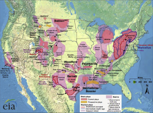
Figure 3.13 Shale gas basins and play trends, the continental United States. From U.S. Energy Information Administration, 2011.
Canada got into shale gas business much later than the United States. Only after 2000s that Candian shale plays have been systematically exploited. Hamblin (2006) reviewed 50 shale units in seven major regions of Canada to produce a geographic inventory of significant shale potential across the country (Figure 3.14–3.17). He concluded that many of these shales have interesting geological characteristics that make them worthy of further investigation. Hamblin (2006) judged the following shale gas units as worthy of concerted geological examination:
• Middle to Upper Ordovician of Appalachian Mountains, St. Lawrence Platform, and Anticosti Island (Utica, Collingwood, Blue Mountain);
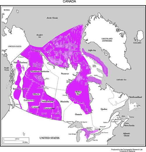
Figure 3.14 Shale plays in Atlantic Canada, Quebec, Ontario, and Hudson margin. From Hamblin, 2006.
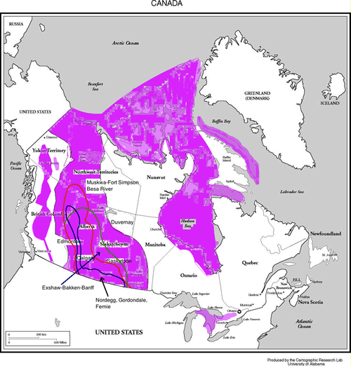
Figure 3.15 Shale gas play areas, western Canada Paleozoic and Mesozoic passive margin platform. From Hamblin, 2006.
• Middle and Upper Devonian of western Alberta, northeastern BC, Liard Basin, and Mackenzie Corridor (Horn River, Muskwa, Imperial, Fort Simpson, Besa River);
• Lower to Middle Triassic of northwestern Alberta and northeastern BC (Montney, Doig);
• Jurassic of western Alberta and northeastern BC (Nordegg, Gordondale, Fernie); and
• Middle-Upper Cretaceous of Alberta, Saskatchewan, and Manitoba (Colorado).
Figure 3.18 shows all North American shale play areas. While broadly distributed, North American shale gas basins generally follow a trend of thrust belts and a Mississippian/Devonian shale fairway from Western Canada and into the Western, Southern, and Eastern United States. The Laramide Thrust Belt bounds the Horn River and Montney Play in British Columbia and Alberta, as well as many of the Western US shale gas fields, including Jonah and Pinedale. Starting in South Texas, the Ouchita Thrust Belt bounds Southern US gas basins, including Eagle Ford, Barnett, Woodford, Haynesville and Fayetteville. Finally, the merger of the Ouchita and Appalachian Thrust Belts define the broad extents of the Marcellus shale gas basin.
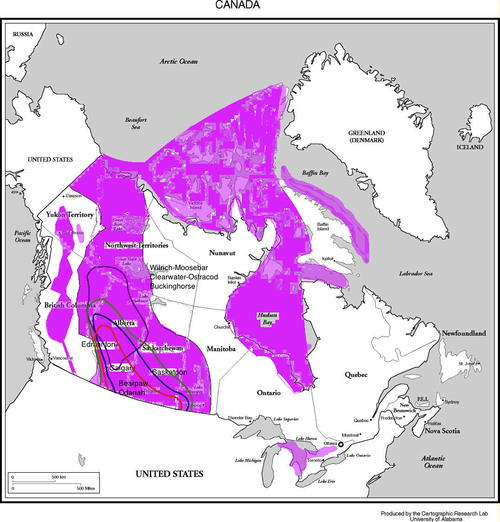
Figure 3.16 Shale gas play areas, western Canada Mesozoic foreland basin. From Hamblin, 2006.
North American shale gas reservoirs currently rank as 6 of the largest 22 global gas fields (Figure 3.19), based upon estimated recoverable reserves, with average recovery factors of about 20%. This recovery factor can be increased significantly if new techniques for recovery are used. Enhanced gas recovery schemes, not yet commercially applied, offers great promises for the future. In the mean time, 3D seismic, microseismic, Formation MicroImager/Formation MicroScanner and other measurements, are pivotal in unlocking North American gas supplies for the decades ahead.
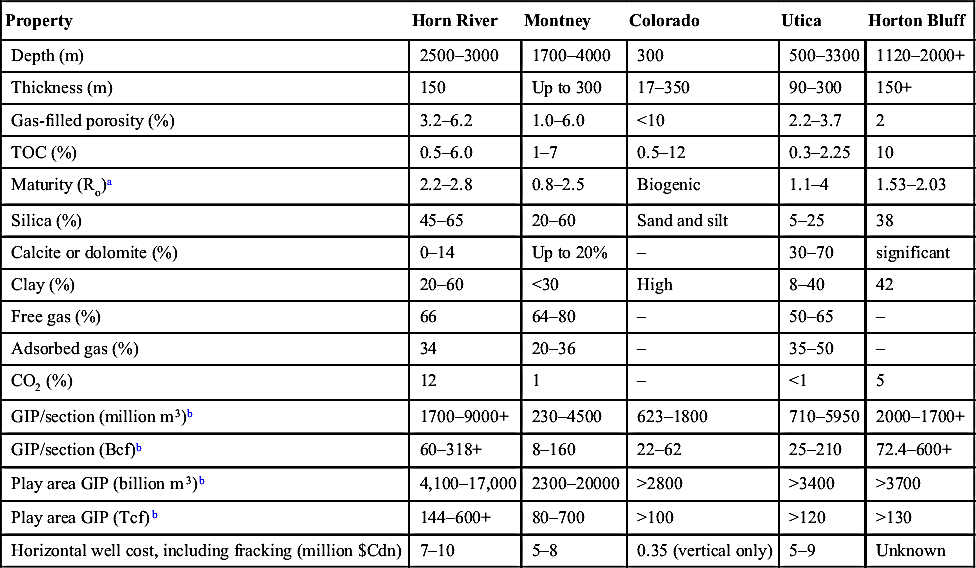
Tables 3.3 and 3.4 shows some of the main features of North American shale plays. Note how reservoir properties vary in such a way that production features are not amenable to Darcian correlation. Further complication arises from the variability in fracturing as well as development of horizontal wells. Surprisingly, after nearly 30 years of development and over 10,000 wells, wellbore lengths and completions parameters in the Barnett Shale of Texas can vary by factors of two or more—pointing to the challenge and non-uniqueness of production optimization (Website 4).
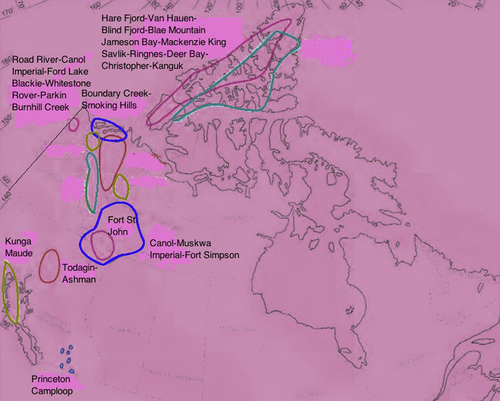
Figure 3.17 Shale gas play areas, Northwest Territories, Arctic Islands, and intermontane basins of BC. From Hamblin, 2006.
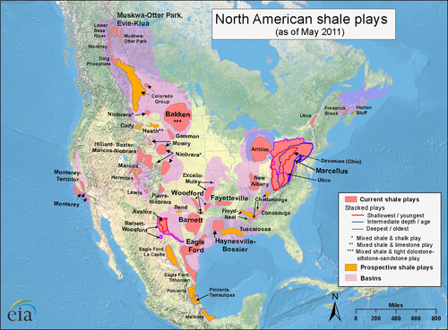
Figure 3.18 North American shale gas basins.
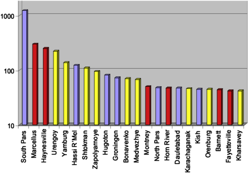
Figure 3.19 World's largest proven gas reservoirs.
At present, the overall effort has been to identify shale gas “sweet spot” and avoid “dead zones.” Accordingly, multilaterals as well fracturing techniques are designed to maximize access to “sweet spots.” Following is a description of several shale plays of the United States and Canada along with their characteristic features.
Barnett Shale—Fort Worth Basin: These reservoirs are most suitable for production through horizontal wells with multistage completions. The Mississippian Barnett Shale averages 300 ft in thickness, at an average depth of about 7500 ft, with average porosities of 6% and low permeabilities of 250nD. Average well production reaches 2.65 Bcf, with initial production rates of up to 13 mmcf/day. Seismic data is generally of moderate quality, but is essential for tracking the key bounding horizons and identifying karst “collapse chimneys” that can cause severe decline in individual well production. This is shown in Figure 3.20. In addition, vitrinite reflectance averages 2% in the Barnett, but drops down in the northern basin.
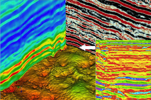
Figure 3.20 Barnett seismic, inversion and surface showing karst collapse chimneys. (Modified from Devon Energy, website 4).
Table 3.3
Shale Gas Reservoir Properties
| Shale Play | Barnett | Haynesville | Marcellus | Horn River | Eagle Ford |
| Age | Mississippian | Upper Jurassic | Middle Devonian | Upper Devonian | Cretaceous |
| MYA | 340 | 170 | 385 | 370 | 100 |
| Total area size (sq mi) | 50,000 | 9000 | 95,000 | 5000 | 1350 |
| Total gas (Tcf) | 327 | 717 | 1500 | 370 | N/A |
| Gas in place (Bcf/sq mi) | 150 | 175 | 200 | 250 | 200 |
| Producible gas (Tcf) | 50 | 251 | 356 | 47 | N/A |
| Depth (ft) | 7,500 | 12,000 | 7000 | 8800 | 11,500 |
| Thickness (ft) | 300 | 225 | 350 | 450 | 250 |
| Horizontal well cost ($M) | 2.8 | 7.0 | 3.5 | 7.0 | 4.8 |
| Average EUR (Bcf) | 2.65 | 6.5 | 3.75 | N/A | 5.5 |
| Pressure (psi) | 4000 | 8500 | 4000 | N/A | 5200 |
| Temperature (°F) | 200 | 340 | N/A | 160 | N/A |
| Ro (%) | 2 | 2.2 | 1.3 | 2.5 | 1.5 |
| TOC (%) | 4.5 | 3 | 3.3 | 3 | 4.5 |
| Porosity (%) | 6 | 10 | 8 | 3 | 11 |
| Matrix permeability (nD) | 250 | 658 | 1000 | 230 | 1100 |
| Pressure gradient (psi/ft) | 0.53 | 0.95 | 0.4 | 0.6 | 0.65 |
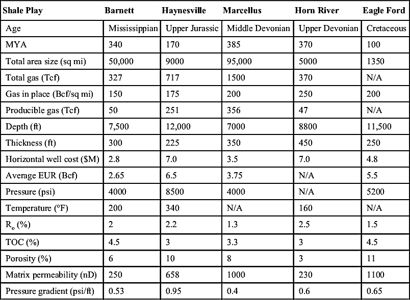
From Website 4.
Table 3.4
| Property | Horn River | Montney | Colorado | Utica | Horton Bluff |
| Depth (m) | 2500–3000 | 1700–4000 | 300 | 500–3300 | 1120–2000+ |
| Thickness (m) | 150 | Up to 300 | 17–350 | 90–300 | 150+ |
| Gas-filled porosity (%) | 3.2–6.2 | 1.0–6.0 | <10 | 2.2–3.7 | 2 |
| TOC (%) | 0.5–6.0 | 1–7 | 0.5–12 | 0.3–2.25 | 10 |
| Maturity (Ro)a | 2.2–2.8 | 0.8–2.5 | Biogenic | 1.1–4 | 1.53–2.03 |
| Silica (%) | 45–65 | 20–60 | Sand and silt | 5–25 | 38 |
| Calcite or dolomite (%) | 0–14 | Up to 20% | – | 30–70 | significant |
| Clay (%) | 20–60 | <30 | High | 8–40 | 42 |
| Free gas (%) | 66 | 64–80 | – | 50–65 | – |
| Adsorbed gas (%) | 34 | 20–36 | – | 35–50 | – |
| CO2 (%) | 12 | 1 | – | <1 | 5 |
| GIP/section (million m3)b | 1700–9000+ | 230–4500 | 623–1800 | 710–5950 | 2000–1700+ |
| GIP/section (Bcf)b | 60–318+ | 8–160 | 22–62 | 25–210 | 72.4–600+ |
| Play area GIP (billion m3)b | 4,100–17,000 | 2300–20000 | >2800 | >3400 | >3700 |
| Play area GIP (Tcf)b | 144–600+ | 80–700 | >100 | >120 | >130 |
| Horizontal well cost, including fracking (million $Cdn) | 7–10 | 5–8 | 0.35 (vertical only) | 5–9 | Unknown |
Marcellus Shale—Appalachia: This is the largest of the United States shale gas plays and covers nearly 100,000 sq mi in Pennsylvania, Virginia, and New York state. Comparable to the Barnett in depth (7000 ft), thickness (350 ft) and porosity (8%)—permeabilities reaching 1 μD are favorable conditions for as high as 3.75 Bcf/day gas production. Such high productivity is attributed to faults, abundance of fractures, fissures, and variable shale and carbon lithology. Figure 3.21 shows a typical cross section.
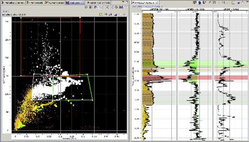
Figure 3.21 Marcellus lithology variations.
Horn River Basin—North-Eastern British Columbia: The unique feature of the Horn River is that it contains multiple prospective shales including the Carboniferous–Devonian Muskwa, Otter Park, Klua, and Evie formations. Prospectivity of these formations vary across the Horn River Basin, leading to alternating or combined completions across the play. The Horn River is a reasonable facsimile of the Barnett, with similar porosities and permeabilities and well depths of about 8800 ft and an average pay zone thickness of 450 ft.
Eagle Ford Shale—South Texas: One of the newest shale gas plays is the Cretaceous Eagle Ford, located in South Texas. It has porosities of 11% and permeability in excess of 1 μD, making it a good candidate for gas recovery. This play is not well studied but initial seismic and microseismic data are encouraging.
In general, Gas shales are source rocks that have not released all of their generated hydrocarbons. In fact, source rocks that are “tight” or “inefficient” at expelling hydrocarbons may be the best prospects for shale gas potential. In this, more than any other factor is the surrounding environment that makes the migration of gas out of the source rock as shale is a reservoir, source rock as well as a trap for natural gas. Most gas is in the adsorbed form, in which gas forms mono- or multilayer. In order to unlock the adsorbed gas, there needs to be a change in either pressure or temperature or both. To date, the main technique for extraction of natural gas from shale gas formations has been through depressurization, which can be achieved by increasing the surface area (horizontal well drilling) and/or by increasing permeability near the wellbore through fracturing.
Unlike tight gas reservoirs, desorption in shale gas would involve separation of gas phase from the bitumen. Recall that shale gas is generated by the following mechanisms:
• primary thermogenic degradation of organic matter;
• secondary thermogenic cracking of oil;
• biogenic degradation of organic matter.
Mono- or multilayer is formed between adsorbed gas and rock in pores, whereas gas remains in diffused/absorbed forms within bitumen and oil. Free gas in shale gas can remain only in fractures and fissures. A higher amount of free gas results in high production rate in the beginning of the production history. As this gas is exhausted, the production rate declines. Any increase in production rate has to be invoked by pressure or thermal change in the reservoir.
In general, gas shales have much lower permeability than sandstone, limestone, or dolomite. Its effective permeability is several orders of magnitude less than 0.1 mD, the cutoff point for “unconventional” reservoirs. With the exception of a few profusely fractured shale gas reservoirs (e.g., Antrim shale in the Michigan basin of the United States), they are in need of artificial stimulation, such as fracturing.
3.3.4. Gas Hydrate Methane
Gas hydrates are unlike any other form of unconventional gas reservoirs. The process of hydrate formation is unique as it involves the trapping of methane molecules directly within water body. Even though biogenic in its root, methane gas is purified during the process of hydrate formation.
Gas hydrate and its potential for generating energy-giving methane is a topic of research that is only a few decades old. Gas hydrates are not like ice, do not melt; they feel more like Styrofoam. Gas hydrates can burn pure methane safely, even inside of house or a meeting room.
Research on methane hydrate has increased in the last few years, particularly in countries such as Japan that have few native energy resources. As scientists around the world learn more about this material, new concerns surface. For example, ocean-based oil-drilling operations sometimes encounter methane hydrate deposits. As a drill spins through the hydrate, the process can cause it to dissociate. The freed gas may explode, causing the drilling crew to lose control of the well. This concern is similar to CBM that posed hazards to miners long before assuming its potential as an energy source.
Another concern is that unstable hydrate layers could give way beneath oil platforms or, on a larger scale, even cause tsunamis. While research in hydrate has many facets, most research has focused on understanding how hydrates form, and little on how hydrate can be used to unlock huge amount of clean methane. Recent work of the Livermore-USGS team shed new light on hydrate formation. They attempted an entirely new procedure. They mixed sieved granular water ice and cold, pressurized methane gas in a constant–volume reaction vessel and slowly heated it. Warming started at a temperature of 250 K with a pressure of about 25 MPa. The reaction between methane and ice started near the normal melting point of ice at this pressure (271 K) and continued until virtually all of the water ice had reacted with methane, forming methane hydrate. The team studied the resulting material by X-ray diffraction and found pure methane hydrate with no more than trace amounts of water. As a result, they developed low-porosity, cohesive samples with a uniformly fine grain size and random crystallographic grain orientation. This laboratory synthesis is useful for shedding light on actual process of natural hydrate formation. It is also remarkable that the study showed that the ice did not liquefy as it should have when its melting temperature was reached and surpassed. In fact, methane hydrate was formed over a period of 7 or 8 h, with the temperatures inside the reaction vessel reaching 290 K before the last of the ice was consumed.
In other experiments conducted with neon, no hydrate was formed. Under otherwise identical experimental conditions, the ice melted as it should, showing reversibility of the process. Other experiments replaced the methane with both gaseous and liquid carbon dioxide, which formed a hydrate. Here the superheating phenomenon reappeared, indicating that it is not unique to methane hydrate. It appears that formation of hydrate and the thermal hysteresis observed are related to water. Water forms such hydrates with methane and carbon dioxide but does not form with neon or other inert gases that are not directly involved with organic matter.
Another surprising finding was when the team studied the formation of dissociation of gas hydrates. After the samples were created, the pressure was reduced to 0.1 MPa, the pressure at sea level. They did this in two ways: by slow cooling and depressurization and by rapid depressurization at a range of temperatures. The compound decomposed to ice and gas as expected in all experiments except those that involved rapid depressurization at temperatures from 240 to 270 K. In these experiments, the team found yet another surprise. Even after the pressure drop, the methane hydrate was “preserved” as a compound for as long as 25 h before it decomposed. This behavior may have implications for future exploitation of the material. Preserving the mixed hydrates may be possible at an easily accessible temperature, just a few degrees below ice's melting temperature.
In another series of experiments, the team is looking at the strength of gas hydrate samples in various temperature and pressure scenarios. Results of these experiments may indicate the possible effects that stresses from gravity, tectonic activity, or human disturbance might have on gas hydrate deposits. Thus far, the team has found that water ice and methane hydrate have about the same strength at very low temperatures of 180 K and below. But the hydrate is much stronger than ice at temperatures of 240 K and above. The most recent data indicate that methane hydrate is several times stronger than ice, although not as strong as rocks.
Figure 3.22 shows how methane seeps through a marine environment and forms hydrates. In both marine and arctic environment, hydrates can form. Before forming solid hydrates, the system is purged of salinity as well as contaminants. The hydrate may mix with solid depositions, but does not lose its potential as an energy retainer. This is evidenced in the phase diagram in Figure 3.23.
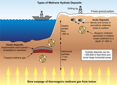
Figure 3.22 Hydrate formation in natural environment.
Figure 3.23 shows the phase diagram of free methane gas and methane hydrate for a pure watered and pure methane system. The addition of NaCl to water shifts the curve to the left. Adding CO2, H2S, C2H6, C3H8 to methane shifts the boundary to the right, thereby increasing the area of the hydrate stability field. It means, natural purification of methane before hydrate is formed.
Methane hydrate is a cage-like lattice of ice inside which are trapped molecules of methane, the chief constituent of natural gas. If methane hydrate is either warmed or depressurized, it will produce natural gas that is pure and ready to burn. When brought to the earth's surface, one cubic meter of gas hydrate releases 164 m3 of natural gas. Hydrate deposits may be several hundred meters thick and generally occur in two types of settings: under Arctic permafrost, and beneath the ocean floor. Methane that forms hydrate can be both biogenic, created by biological activity in sediments, and thermogenic, created by geological processes deeper within the earth. Hydrates contain the most naturally purified methane available on earth. The processing involves water, thereby making the final product most suitable for human energy consumption.
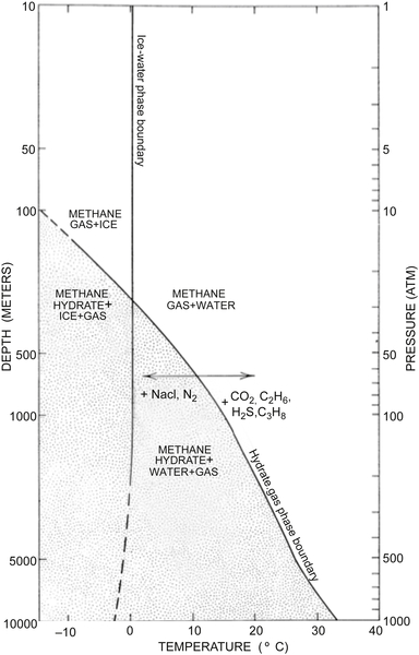
Figure 3.23 Phase diagram of brine and methane. From Kvenvolden, 1993.
During gas hydrate formation, water molecule crystallize into cubic lattice structures (Figure 3.24).
Figure 3.24 shows the structure of gas hydrates. The rigid cages in the figure are composed of hydrogen-bonded water molecules and each cage contains a methane molecule. During the formation process, hydrate crystals expel salt ions from the crystal structure. Measurements of chlorine in gas hydrate samples indicate far less concentration of salt than sea water (Kvenvolden and Kastner, 1990). The salt concentration of around 2% represents the salinity level of normal drinking water in contrast to some 20% concentration in sea water.
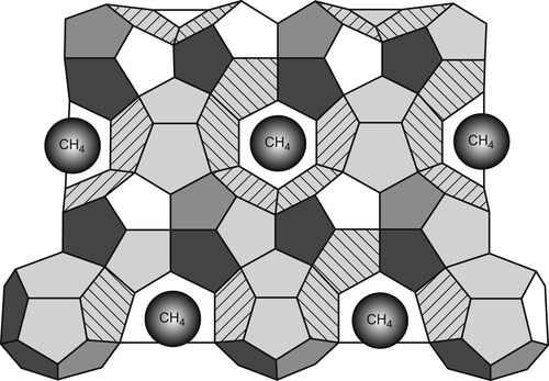
Figure 3.24 Molecular structure of hydrate.
The U.S. Department of Energy methane hydrate program aims to develop the tools and technologies to allow environmentally safe methane production from arctic and domestic offshore hydrates. This research is in its nascent state and is discussed below in order to familiarize the reader of the unknown nature of hydrate. The program includes research and development in the following areas:
Production feasibility: Methane hydrates occur in large quantities beneath the permafrost and offshore, on and below the seafloor. DOE R&D is focused on determining the potential and environmental implications of production of natural gas from hydrates. Figure 3.25 shows the phase diagram for the two types of hydrates.
DOE's methane hydrate program is focused on developing the technology and knowledge that will allow industry to commercialize methane hydrate production. DOE's field programs are focused on the Alaska North Slope and offshore Gulf of Mexico as both contain prolific known petroleum systems conducive to the formation of gas hydrates, as well as a wealth of information and infrastructure developed during decades of industry hydrocarbon exploration. The well-delineated gas hydrate occurrences on the Alaska North Slope provide relatively low-cost opportunities to conduct extended duration field production trials. The Gulf of Mexico provides a laboratory for testing gas hydrate exploration technology and providing an initial confirmation of the scale of marine gas hydrate occurrence in the United States.
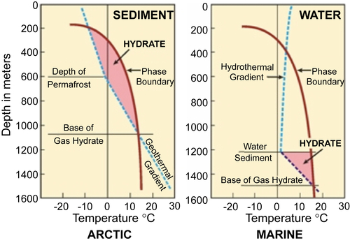
Figure 3.25 Phase diagram of hydrate under arctic and marine environments.
Research and modeling: DOE is studying innovative ways to predict the location and concentration of subsurface methane hydrate before drilling. DOE is also conducting studies to understand the physical properties of gas hydrate-bearing strata and to model this understanding at reservoir scale to predict future behavior and production. Research is focused on understanding the physical and chemical nature of gas hydrate-bearing sediments.
Gas hydrate characterization in the Gulf of Mexico, Scripps Institute of Oceanography: Investigates the feasibility of using marine electromagnetic surveying as a tool for characterizing and quantifying the occurrence of hydrate in the seafloor section.
Electrical resistivity investigation of gas hydrate distribution in Mississippi Canyon Block, Baylor University: Will evaluate the direct-current electrical resistivity method for remotely detecting and characterizing the concentration of gas hydrates in the deep marine environment.
Gas hydrate research in deep sea sediments, Naval Research Lab: Develops and tests a bottom-mounted seismic source for mapping gas hydrates in marine environments.
Detection and production of methane hydrate, Rice University: Investigates the local and regional variations in methane hydrate deposits, where differences in in situ concentrations are relevant to the importance of gas hydrate as a resource, a geohazard, and a factor in the carbon cycle.
Heat flow and gas hydrates on the Continental Margin of India, University of Oregon: Investigates the relationship of residual heat flow anomalies to fluid flow and gas hydrate distribution in the subsurface.
Mechanisms leading to coexistence of gas and hydrate in ocean sediments, University of Texas at Austin: Understands the manner in which methane is transported within the hydrate stability zone and consequently, the growth behavior of methane hydrates at both the grain scale and bed scale.
Methane recovery from hydrate-bearing sediments, Georgia Institute of Technology: Develops observational and experimental data relative to the basic mechanisms at work in a methane hydrate reservoir that is under production.
Natural Gas hydrates in permafrost and marine settings—resources, properties, and environmental issues, U.S. Geological Survey: assist in characterizing and modeling arctic and marine methane hydrates, and participate in design and execution of field studies.
Modeling activities are centered on a multinational effort to optimize computer codes for simulating methane hydrate reservoir behavior. The code comparison study compares the results of simulations of field and laboratory data sets by several commercial and public methane hydrate reservoir simulators. This allows for improvement in the models and also generates a repository of simulations of hydrate formation and dissociation behavior. Research at DOE national labs provides laboratory data on methane hydrate formation and dissociation that is used to enhance the models.
Laboratory studies in support of characterization of recoverable resources from methane hydrate deposits, Lawrence Berkeley National Lab: Studies in support of reservoir simulation include hydrologic measurements, combined geomechanical/geophysical measurements, and synthetic hydrate formation studies.
Formation and dissociation of methane hydrates, National Energy Technology Lab: Validates results from reservoir simulations relative to hydrate re-formation during gas production, gas migration within hydrate-bearing sediments, and carbon dioxide–methane exchange within sediments.
Climate change: DOE is studying the role of methane hydrate formation and dissociation in the global carbon cycle. Another aspect of this research is incorporating gas hydrate science into climate models to understand the relationship between global warming and methane hydrates.
Methane hydrates store huge volumes of methane formed by the bacterial decay of organic matter or leaked from underlying oil and natural gas deposits. The active formation of methane hydrates in the shallow crust prevents methane, a greenhouse gas, from entering the atmosphere. On the other hand, warming of arctic sediments or ocean waters has the potential to cause methane hydrate to dissociate, releasing methane into the deepwater sediments, the ocean or atmosphere. DOE is conducting research to understand the mechanisms and volumes involved in these little-studied processes.
DOE environmental and climate change research projects related to Arctic methane hydrate deposits include:
Characterization of methane degradation and methane-degrading microbes in Alaska coastal waters, University of Delaware: Studies methane degradation and methane-degrading microbes in order to improve predictive models of methane fluxes in the Arctic.
Source characterization and temporal variation of methane seepage from thermokarst lakes on the Alaska North Slope in Response to Arctic climate change, University of Alaska Fairbanks and U.S. Geological Survey, Woods Hole, Massachusetts: Characterize the source, magnitude, and temporal variability of methane seepage from thermokarst lakes in the Alaskan North Slope, and to assess the vulnerability of these areas to ongoing and future arctic climate change.
Interrelation of global climate and the response of oceanic hydrate accumulations, Lawrence Berkeley National Lab and Los Alamos National Lab and U.S. Geological Survey's Study of Beaufort Sea Hydrate DOE environmental and climate change research projects related to marine or global methane hydrate deposits include:
Gulf of Mexico gas hydrates seafloor observatory project, University of Mississippi Center for Marine Resources and Environmental Technology: The Gulf of Mexico-Hydrate Research Consortium (GOM-HRC) is developing a seafloor station to monitor hydrates in situ.
Integrating natural gas hydrates in the global carbon cycle, University of Chicago: Develops a two-dimensional, basin-scale model for the deep sediment biosphere with methane dynamics to understand the distribution of hydrates on the seafloor and their vulnerability to warming of the deep ocean, thus integrating methane hydrates into the global carbon cycle.
Remote sensing and sea-truth measurements of methane flux to the atmosphere, Texas A&M University, Corpus Christi: Improves estimates of methane flux from submarine seeps and associated gas hydrate deposits on continental margins by compiling a remote sensing inventory of active gas and oil vents.
Assessing the efficacy of the aerobic methanotropic biofilter in methane hydrate environments, University of California, Santa Barbara: Assesses the efficacy of aerobic methanotrophy in preventing the escape of methane from marine, hydrate-bearing reservoirs to the atmosphere and ultimately to better define the role of aerobic methanotrophy in the global carbon cycle.
Interrelation of global climate and the response of oceanic hydrate accumulations, Lawrence Berkeley National Lab and Los Alamos National Lab: Investigates the effect of rising water temperatures on the stability of oceanic hydrate accumulations, and estimate the global quantity of hydrate-originating carbon that could reach the upper atmosphere and its impact on global climate.
Natural gas hydrates in permafrost and marine settings—resources, properties, and environmental issues, U.S. Geological Survey: Studies the links between Late Pleistocene to contemporary climate change and the state of the gas hydrate reservoir in high-latitude regions, specifically the US Arctic.
International collaboration: International collaboration continues to be a vital part of the program since gas hydrates represent research challenges and resource potential that are important on a global scale.
In 1982 the multinational Deep Sea Drilling Program recovered the first subsea substantial methane hydrate deposits, which spurred methane hydrate research in the United States and other countries. The successor programs, the Ocean Drilling Program (ODP) and the Integrated Ocean Drilling Program (IODP) sampled hydrate deposits off Oregon (ODP 204, 2002) and in the Cascadia Margin off Vancouver Island, Canada (ODP 146, 1992 and IODP 311, 2005). In the Atlantic Ocean off the United States, ODP Leg 146 sampled hydrate deposits on the Blake Ridge and Carolina Rise in 1995.
International cooperation helps scientists in the United States and other countries expand their understanding of the variety of naturally occurring methane hydrate deposits and develop expertise in sampling and measurement techniques. Although methane hydrate deposits are inferred to exist on all continental shelves, only a few sites have been drilled and logged or cored, which makes this information valuable to all scientists. DOE is participating as a steering committee member in a global assessment of methane hydrates in the natural environment, led by the United Nations Environment Programme. Information on the assessment is available at http://www.methanegashydrates.org.
Because of the broad level of international cooperation, information is available on research programs and sampling expeditions for Canada, India, China, Japan, and Korea. Additional information about specific international methane hydrate research expeditions is available in numerous articles in the newsletter, Fire in the Ice.
Overall, gas hydrate methane is an excellent source of natural gas. Most commonly found hydrates (e.g. Gulf of Mexico) is mostly microbial with others being thermogenic. In these cases, 99% of gas is methane. Gas hydrates associated with mud volcanoes in the Caspian Sea contain hydrocarbon gases with 59–96% methane having carbon isotopic compositions of 44.857.3%. These are essentially thermogenic methane.
3.4. Global Warming and Natural Gas
Previous sections confirm that natural gas from unconventional sources are the most naturally processed energy source. Often, natural gas is considered to be “lesser evil.” This results from years of campaign that is devoid of scientific premises. Aggressive development of petroleum resources has been curtailed by the recent “awareness” of environmental consequences of petroleum production and utilization. “Petroleum production and utilization is the cause for environmental disaster” is the predominant theme today (Picture 3.2). Yet, petroleum fluid is the 2nd most abundant fluid (second only to water) on earth and presents the most potent purely naturally processed energy source. Also, petroleum contains the most amount of carbon, the essential ingredient of life on earth.

Picture 3.2 “Petroleum is dirty, anything else is clean” is the most dominant environmental theme today.
Despite the bad name, oil and gas continue to be the most dominant energy provider of the world. For many decades, oil production from all regions have been increasing steadily. World oil production increased by 1.9 million bbl/day in 2012, more than double the growth of global consumption. US output grew by 1 million bbl/day, the largest increase in the world and in the country's history. Interestingly, global oil consumption grew at a less steep pace and Europe and North America marked decline in oil consumption over the past years. Figure 3.26 shows the history of production from various regions.
Figure 3.27 shows future projections of accelerated production from OPEC countries. OPEC production in the reference case grows from 35 million bbl/day in 2011 to 48 million bbl/day in 2040. Although the OPEC resource base is sufficient to support much higher production levels, the OPEC countries have an incentive to restrict production in order to support higher prices and sustain revenues in the long term. The role of OPEC will become more intense after 2020. The reference case assumes that OPEC will maintain a cohesive policy of limiting supply growth, rather than maximizing total annual revenues. The reference case also assumes that no geopolitical events will cause prolonged supply shocks in the OPEC countries that could further limit production growth. The uncertainty in the oil pricing due to political instability cannot be ruled out and is likely to be a major factor that cannot be predicted. Figure 3.28 shows how previous oil market has been affected by political events.
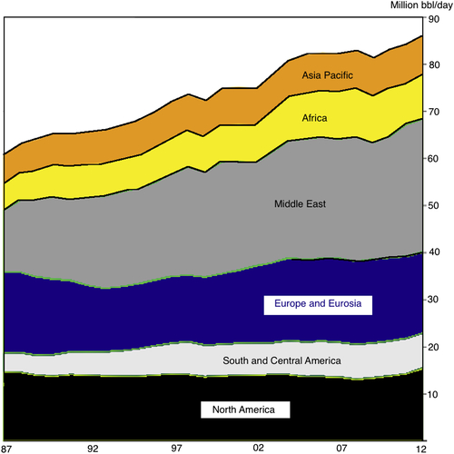
Figure 3.26 Oil productions (million bbl/day) for various regions. Redrawn from Courtesy BP Outlook, 2013.
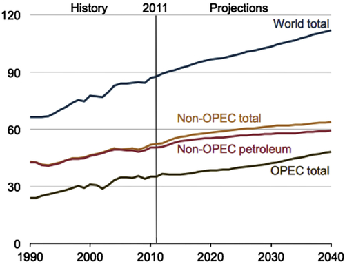
Figure 3.27 Future prediction of global oil production. EIA, 2013 annual report.
The growth in non-OPEC production results primarily from the development of new fields and the application of new technologies, such as enhanced oil recovery, horizontal drilling, and hydraulic fracturing, which increase recovery rates from existing fields. The average cost per barrel of non-OPEC oil production rises as production volumes increase, and the rising costs dampen further production growth.
Non-OPEC production of other liquids grows from 1.8 million bbl/day in 2011 to 4.6 million bbl/day in 2040, as Brent crude oil prices remain sufficiently high to make other liquids production technologies economically feasible. Non-OPEC liquids production in the reference case totals 58 million bbl/day in 2020, 61 million bbl/day in 2030, and 64 million bbl/day in 2040.
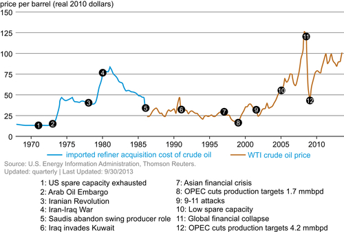
Figure 3.28 Oil price and world political events.
The apparent “vilification” of petroleum activities did not change the prediction that petroleum resources will continue to dominate the world energy scenario for many decades to come. However, at the same time, few have countered the environmental arguments with proper science. Instead, there has been contradictory evidence and argument shifting blames on everything but the process that “refines” petroleum. The debate has taken an unprecedented acrimony between supporters and detractors of petroleum industry. The topic is global warming and the two camps have been entrenched in their respective positions with utmost rigidity. These positions being: (1) There is no global warming, (2) Carbon is the enemy. Figure 3.29 shows the weather map of June, 2013 that reported record breaking temperature in Alaska.
This event prompted detractors to quickly condemn all forms of petroleum production and attacking petroleum supporters as “flat earth theoretician.”
Within a few months, another report came up stating that Antarctic has an unprecedented build up of ice, prompting supporters to dismiss global warming as a “myth.” Figure 3.30 shows the buildup of ice in the Antarctic as reported in the Fall of 2013. Figure 3.31 shows the temporal extent of the ice buildup.
Figure 3.29 June 18, 2013 saw record breaking heat in Alaska.
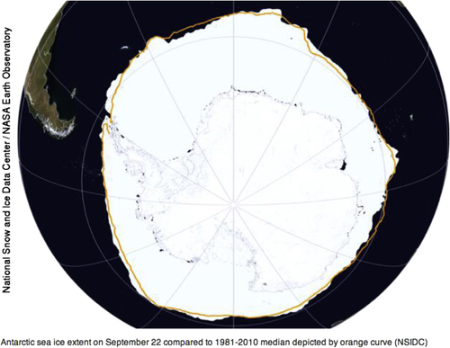
Figure 3.30 September 22, 2013 picture shows unprecedented ice buildup in the Antarctic.
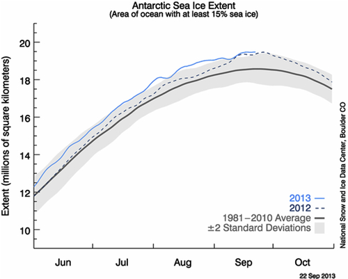
Figure 3.31 Recent report shows unprecedented buildup of ice in the Antarctic.
This fueled the notion that Sorokhtin et al. (2007) were correct in predicting we are actually in the midst of a global cooling. Fluctuations in CO2 leads to fluctuations in global temperatures (Figure 3.32). This figure is used to claim that we are in fact in a cooling cycle if we consider natural phenomena in the geological time scale. These supporters argue that ice and soil cores the earth has gone through many up and downs. We have surpassed 400 ppm of CO2 now which we have many times before. They claim that oxygen levels were extremely high during the ages of dinosaurs. Some scientists point to the Sun for the increase in temperatures, which they say is happening to all the inner orbit planets. The Sun is hitting maxima now but the hope is that it will stabilize in time before the earth becomes in habitable. All these come from the premise that the Sun, Earth, etc., are all part of a random process. What is rarely talked about is that such “natural phenomena” have been severely altered because of the emergence of artificial materials. When Freon was just introduced, it was said, there is no way it can make a dent in the atmosphere, the emission being so insignificant. After all, they argued, nature is too vast to be impacted by human activities. At present it is said, we only burn 100 million bbl of oil, a peanut compared to the total CO2 emission by the entire biomass of this planet. New science does not account for the theory that these artificially generated CO2 are to the earth what cancer causing chemicals are to the human body.
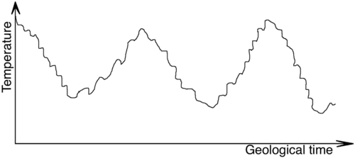
Figure 3.32 In geological scale, the current epoch is actually in a cooking cycle.
The opponents of petroleum activities claim that because CO2 is the source of global warming, any process that uses carbon is harmful and must be eliminated. This fateful conclusion that “Carbon is the enemy” is deconstructed by asking the pointed question: “Are you saying CO2 that is the only source of carbohydrate is a problem while nuclear is not?” In order to remove the paradox, one must invoke a paradigm shift in the first premise. It has been done by Islam et al. (2010) in the following sequence.
1. Nature is perfect. This is the major premise. It means only natural is sustainable and readily accepted by nature.
2. In order to posit a minor premise, it is asked: What is natural? The answer is put as a minor premise.
3. Then, an axis is formed with the major premise as the source and minor premise as the other point of the axis. That created a unique set of scaling laws.
4. With this set of scaling laws (or standards), it can be concluded that
a. CO2 is not the problem;
b. It is the artificial (not naturally occurring) additives that are the problem. These polluted CO2 are the source of global warming.
If natural, excess CO2 would increase vegetation, thereby bringing down global temperature and increasing O2 supply to the ecosystem.
This is captured in the Figure 3.33 that shows in exaggerated scale what happened ever since artificial chemicals have been in use for refining crude oil.
The millions of barrels are burnt everyday that emit large amount of artificial CO2 that cannot be absorbed by the ecosystem. This is the type of CO2 that contributes to the rapid increase in CO2 in the atmosphere, despite that fact that natural carbon dioxide in the atmosphere is decreasing, albeit very slightly. Note that the overall rise of the CO2 content or the global temperature is conflated by most supporters as “natural phenomena” that one should be able to observe as an extension of the variation in geological time. The inability to distinguish between natural and artificial (polluted with additives) CO2 has made it impossible to pin point the cause of global warming. It also turns out that the same additives are all carcinogenic, thereby creating strong correlation between the usage of petroleum products with devastating impact on human health.
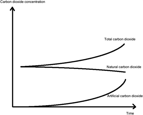
Figure 3.33 Schematic of temporal change in various types of carbon dioxide.
As for the controversy regarding the buildup of extra ice in the Antarctic region is explained as an effect of global warming. The following depiction (Figure 3.34) by Argonne National laboratory explains such a buildup in terms of global ocean circulation between deep, colder water and warmer, surface water, strongly influencing regional climates around the world (NASA, 2004). It was in fact predicted that the entire North America and Western Europe would plunge into ice age. This gave a significant fighting weapon to the detractors of petroleum activities, while the other group avoided giving reference to it until the report of massive build up of ice in the Antarctic was reported (NASA, 2013a). For them, it is a clear evidence that global warming is a hoax.
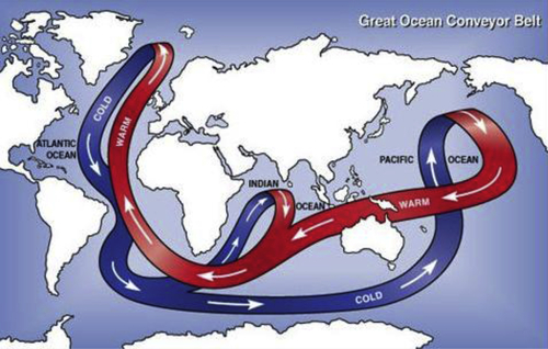
Figure 3.34 As early as 2004, NASA raised the alarm that global warming can lead to more ice buildup in the Antarctic.
In 2012, NASA raised alarm regarding north pole ice being sixth lowest in recorded history (NASA, 2012). In 2013, NASA recorded highest accumulation of ice in the Antarctic (NASA, 2013).
However, another report of NASA (2013b) showed loss of ice in the North pole. This report was not used by the supporters of petroleum activities.
While the diminishing north pole ice can be linked to “warming,” the simultaneous rise in water temperature and build up of record level of ice in Antarctic as well as record breaking high temperature in Alaska created the so-called “Arctic sea ice paradox.” (Figure 3.35) Similar to numerous other paradoxes that have crippled New Science, this paradox cannot be removed unless contradictions at the fundamental levels are removed. Once again, one is faced with distinguishing between types of ice that emerge from different sources. For instance, continental ice is different from sea ice. Continental ice is formed by the gradual deposition, buildup, and compaction of snow, resulting in ice that is hundreds to thousands of meters thick. This ice stores and releases freshwater that can affect the ecosystem for thousands of years. On the other hand, sea ice is a thin layer (not more than 2 m) of ice that forms on the surface of the ocean when the atmospheric temperature is below the freezing point. Once ice is formed, it acts as an insulator and the sea temperature is conserved. This is necessary for the aquatic life to be protected. The sea ice is mobile and transitory. It can revert to water as the prevailing conditions change. From there sea ice can move with the winds and currents, continuing to grow both by freezing and through collisions (between the floes that make up the ice cover). When the atmosphere, and/or ocean is suitably warm again, such as in spring or if the sea ice has moved sufficiently towards the equator, then the sea ice melts again. In the Antarctic, approximately 80% of the sea ice area grows each autumn to winter and decays each spring to summer. This annual expansion–contraction from about 4 to 19 million square kilometers is one of the greatest seasonal changes on the earth's surface.

Figure 3.35 The diminishing ice in the North pole has given detractors weapon for an argument to curtail petroleum activities.
In addition, difficulties arise from the false estimation of volume from the area that can be easily monitored. However, monitoring of depth is far from accurate when it comes to sea ice.
In 2013 winter, the Antarctic sea ice coverage was reported to be 3.6% above the winter average calculated from 1981 to 2010, calling for fresh debate on global warming.
This continues a trend that is weakly positive and remains in stark contrast to the decline in Arctic summer sea ice extent (2013 was 18% below the mean from 1981 to 2010). Nobody being able to conduct an accurate heat balance, it becomes anyone's guess as to what conclusion should be drawn from these observations. In this the 2004 NASA model for hot and cold stream circulation only explains part of the observations. Furthermore, any density variation of sea ice, along with spatial variation can throw the heat balance calculations. If the global water temperature does go up, it would correspond to retention of more heat in a typical three-layer model as shown in Figure 3.36. Such change in water temperature will affect both the density and areal extent of sea ice.
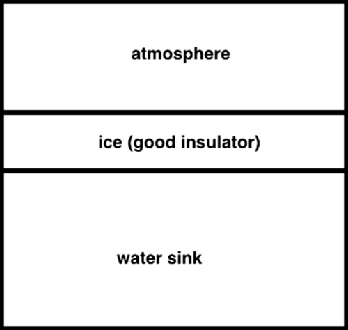
Figure 3.36 Water represents a gigantic heat sink that can store enough heat to stabilize the global temperature in the long term.
Other factors involve ocean/ice interactions, compositional change in atmosphere, wind velocity, all of which will have possible contradictory impacts on the sea ice. Overall, water is an excellent heat sink. Warm water means a great amount of heat loss, which can translate into a huge amount of ice formation. Ice being a great insulator, the atmosphere is not affected by the heating phenomena.
3.5. Distinguishing Features of Unconventional Reservoirs
Even though different forms of unconventional reservoirs are lumped under the title “Unconventional reservoirs,” they have distinguishing features that separate them from each other. On the other hand, they all share certain features that are different from those of conventional reservoirs. In general, it is understood that the differences between conventional and nonconventional lie within the following:
• low-permeability structure itself: this is the most important feature of unconventional reservoirs. Even though the permeability value cut off point is set at 0.1 mD arbitrarily, the fact remains that the matrix permeability of unconventional reservoirs is less than 0.1 mD. Because modern day petroleum engineering is based on Darcy's equation that puts permeability as the most important parameter governing flow rate, the demarcation based on permeability is understandable.
• response to overburden stress: the peculiar response to overburden gives unique characteristics of unconventional reservoirs, resulting in low permeability, devoid of fractures or the presence of random fracture network (e.g. coalbed).
• impact of the low-permeability structure on effective permeability relationships under conditions of multiphase saturation: this feature results in the presence of “permeability jail”—a range of saturation for which none of the fluid flows.
• entrapment of gas in both adsorbed and adsorbed conditions in the reservoir.
The volume of unconventional gas is much more than the volume of conventional gas. Unlike commonly held perception, this additional volume also represents higher quality of natural gas. The most abundant gas resource, hydrate represents the highest quality gas. CBM also shows equally high quality. Even though tight gas and shale gas composition is relatively ‘impure’, they are naturally processed and if sustainable techniques are used to purify offer the best type of natural energy source. Deconstruction of commonly believed accounting theories showed that the relationship between technical feasibility and economics is a fictitious one. With proper science, the cost of developing larger resources is minimized. A discussion on scientific cause of global warming reveals that natural gas from unconventional resources can help reverse global warming if artificial chemicals are avoided during the gas processing phase.
..................Content has been hidden....................
You can't read the all page of ebook, please click here login for view all page.