
Chapter 7
Overview of Reservoir Simulation of Unconventional Reservoirs
Abstract
Reservoir simulation is the most powerful tool for estimating reserve as well as predicting reservoir performance. However, serious limitations exist in fundamentals of reservoir simulation when it comes to conventional reservoirs. Difficulties exist from data acquisition to applicability of Darcy's law and solution techniques that are applicable only to conventional reservoirs. In this chapter, techniques are shown as to how to gather relevant data for reservoir simulation. Mathematical developments of new governing equations based on in-depth understanding of the factors that influence fluid flow in porous media under different flow conditions are introduced. Behavior of flow through matrix and fractured systems in the same reservoir, heterogeneity and fluid–rock properties interactions, Darcy and non-Darcy flow are among the issues that are thoroughly addressed. It is demonstrated that the currently available simulators only address very limited range of solutions for a particular reservoir-engineering problem. Examples are provided to show how currently used techniques can be adjusted to properly model unconventional reservoirs.
Keywords
Brinkman equation; Forchheimer equation; dual porosity; dual permeability; knowledge modeling7.1. Introduction
In reservoir simulation, the principle of garbage in and garbage out is well known (Rose, 2000). This principle implies that the input data have to be accurate for the simulation results to be acceptable. Petroleum industry has established itself as the pioneer of subsurface data collection (Abou-Kassem et al., 2006). Historically, no other discipline has taken so much care in making sure input data are as accurate as the latest technology would allow. The recent superflux of technologies dealing with subsurface mapping, real-time monitoring, and high speed data transfer is an evidence of the fact that input data in reservoir simulation are not the weak link of reservoir modeling.
However, for a modeling process to be meaningful, it must fulfill two criteria, namely, the source has to be true (or real) and the subsequent processing has to be true (Islam et al., 2010). For unconventional reservoirs, they are both of concern. For instance, most commonly used well log data do not register useful information for unconventional reservoirs, which do not allow invasion of sonic signals, mud filtrate, etc., invalidating some of the well logging techniques. Processing data is also of concern. Unconventional reservoirs require special filtering tools that are not readily available. Some of them are presented in previous chapters of this book.
For reservoir simulation to yield meaningful results, the following logical steps have to be taken.
1. Collection of data with constant improvement of the data acquisition technique. The data set to be collected is dictated by the objective function, which is an integral part of the decision-making process. Decision-making, however, should not take place without the abstraction process. The connection between objective function and data needs constant refinement. This area of research is one of the biggest strength of the petroleum industry, particularly in the information age. Each of the data acquisition tools must be reevaluated for applicability in unconventional reservoirs.
2. The gathered data should be transformed into information so that they become useful. With today's technology, the amount of raw data is so huge that the need for a filter is more important than ever before. However, it is important to select a filter that does not skew data set toward a certain decision. Mathematically, these filters have to be nonlinearized (Islam et al., 2010). While the concept of nonlinear filtering is not new, the existence of nonlinearized models is only beginning to be recognized (Hossain and Islam, 2009).
3. Information should be further processed into “knowledge” that is free from preconceived ideas or a “preferred decision.” Scientifically, this process must be free from information lobbying, environmental activism, and other forms of bias. Most current models include these factors as an integral part of the decision-making process (Eisenack et al., 2007), whereas a scientific knowledge model must be free from those interferences as they distort the abstraction process and inherently prejudice the decision-making. Knowledge gathering essentially puts information into a big picture. For this picture to be distortion free, it must be free from nonscientific maneuvering.
4. Final decision-making is knowledge based, only if the abstraction from step 1 through step 3 has been followed without interference. Final decision is a matter of Yes or No (or True or False, or 1 or 0) and this decision will be either knowledge based or prejudice based. Figure 7.1 shows the essence of the knowledge-based decision-making.
The process of aphenomenal or prejudice-based decision-making is illustrated by the inverted triangle, proceeding from the top down (Figure 7.2). The inverted representation stresses the inherent instability and unsustainability of the model. The source data from which a decision eventually emerges already incorporate their own justifications, which are then massaged by layers of opacity and disinformation.
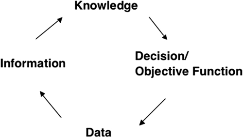
Figure 7.1 The knowledge model.
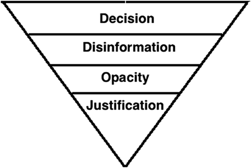
Figure 7.2 The aphenomenal model. After Zatzman, 2012.
7.2. Essence of Reservoir Simulation
Today, practically all aspects of reservoir engineering problems are solved with reservoir simulators, ranging from well testing to prediction of enhanced oil recovery. For every application, however, there is a custom-designed simulator. Even though, quite often, “comprehensive,” “all purpose,” and other denominations are used to describe a company simulator, every simulation study is a unique process, starting from the reservoir description to the final analysis of results. Simulation is the art of combining physics, mathematics, reservoir engineering, and computer programming to develop a tool for predicting hydrocarbon reservoir performance under various operating strategies. The first step in the development of a reservoir simulator is expressing the physical situation in terms of mathematical description. This is called the formulation step. The formulation step outlines the basic assumptions inherent to the simulator, states these assumptions in precise mathematical terms, and applies them to a control volume in the reservoir. Newton's approximation is used to render these control volume equations into a set of coupled, nonlinear partial differential equations (PDEs) that describe fluid flow through porous medium. These PDEs are then discretized, giving rise to a set of nonlinear algebraic equations. Discretization is the process of converting PDEs into algebraic equations. The discretization can be done using the finite difference methods or the approaches based on the variation methods such as finite element methods. However, the most common approach in the oil industry is the finite difference method. To carry out discretization, a PDE is written for a given point in space at a given time level using the Taylor series expansion to convert it in finite difference forms. The choice of time level (old, current, or the intermediate time level) leads to the explicit, implicit, or Crank–Nicolson formulation method. The discretization process results in a system of nonlinear algebraic equations. These equations generally cannot be solved with linear equation solvers and linearization of such equations becomes a necessary step before solutions can be obtained. Well representation is used to incorporate fluid production and injection into the nonlinear algebraic equations. Linearization involves approximating nonlinear terms in both space and time. Linearization results in a set of linear algebraic equations. Any one of several linear equation solvers can then be used to obtain the solution. The solution comprises of pressure and fluid saturation distributions in the reservoir and well flow rates. Validation of a reservoir simulator is the last step in developing a simulator, after which the simulator can be used for practical field applications. The validation step is necessary to make sure that no errors were introduced in the various steps of development and in computer programming.
It is possible to bypass the step of formulation in the form of PDEs and directly express the fluid flow equation in the form of nonlinear algebraic equation as pointed out in Abou-Kassem et al. (2006). In fact, by setting up the algebraic equations directly, one can make the process simple and yet maintain accuracy. This approach is termed the “engineering approach” because it is closer to the engineer's thinking and to the physical meaning of the terms in the flow equations. Both the engineering and mathematical approaches treat boundary conditions with the same accuracy, if the mathematical approach uses second order approximations. The engineering approach is simple and yet general and rigorous.
7.2.1. Assumptions behind Various Modeling Approaches
Reservoir performance is traditionally predicted using three methods, namely, (1) analogical, (2) experimental, and (3) mathematical. The analogical method consists of using properties of a mature reservoir that are similar to that of the target reservoir to predict the behavior of the reservoir. This method is especially useful when there is a limited available data. The data from the reservoir in the same geologic basin or province may be applied to predict the performance of the target reservoir. Experimental methods measure the reservoir characteristics in the laboratory models and scale these results to the entire hydrocarbon accumulation. The mathematical method applied basic conservation laws and constitutive equations to formulate the behavior of the flow inside the reservoir and the other characteristics in mathematical notations and formulations. The two basic equations are the material balance equation or continuity equation and the equation of motion or momentum equation. These two equations are expressed for different phases of the flow in the reservoir and are combined to obtain single equation for each phase of the flow. However, it is necessary to apply other equations or laws for enhanced oil recovery. As an example, the energy balance equation is necessary to analyze the reservoir behavior for the steam injection or in situ combustion reservoirs.
The mathematical model traditionally includes material balance equation, decline curve, statistical approaches, and also analytical methods. The Darcy's law is almost used in all of the available reservoir simulators to model the fluid motion. The numerical computations of the derived mathematical model are mostly based on the finite difference method. All these models and approaches are based on several assumptions and approximations that may cause to produce erroneous results and predictions.
7.2.1.1. Material Balance Equation
Material balance equation is known to be the classical mathematical representation of the reservoir. According to this principle, the amount of material remaining in the reservoir after a production time interval is equal to the amount of material originally present in the reservoir minus the amount of material removed from the reservoir due to production plus the amount of material added to the reservoir due to injection. This equation describes the fundamental physics of the production scheme of the reservoir. Listed below are several assumptions in the material balance equation.
• Rock and fluid properties do not change in space.
• Hydrodynamics of the fluid flow in the porous media is adequately described by Darcy's law.
• Fluid segregation is spontaneous and complete.
• Geometrical configuration of the reservoir is known and exact.
• Pressure–volume–temperature data obtained in the laboratory with the same gas-liberation process (flash vs differential) are valid in the field.
• Material balance equation is sensitive to inaccuracies in measured reservoir pressure. The model breaks down when no appreciable decline occurs in reservoir pressure, as in pressure maintenance operations.
The material balance equation is directly linked to original gas in place. In order to consider production of an unconventional gas reservoir, a sufficient amount of gas in place within the reservoir is a concern. For shale, this usually means it is a hydrocarbon source that generated large volumes of either thermal or biogenic gas. To have generated such large quantities of gas, shale needs to be rich in organic matter, relatively thick, and should have been exposed to source of heat in excess of usual global geothermal gradients. The presence of adsorbed, trapped, and free gases in fractures contributes to the complexity of the problem.
A general equation for calculating gas in place is:
G=A∗h∗ϕ∗Sg
![]() (7.1)
(7.1)
where,
G = Gas in Place
A = Area of the entire trap
h = Average thickness
Sg = Gas saturation
ϕ = Porosity
Note that conventionally, thickness is considered to be net thickness, from which shale breaks are deducted. For analysis of unconventional gas, the total thickness must be considered. Similarly, there cannot be any cutoff point for porosity. For unconventional reservoirs, most porosity occurs within very tight, shale formations and removing those components would seriously falsify total reserve estimate and subsequent prediction.
Total thickness can be calculated from geological estimate of the trap as well as geophysical information. This can later be refined with capillary pressure data. The best estimate of gas saturation is through core analysis.
Organic carbon concentration in the shales is important in deciding its productive potential. Among all shale basins studied here, it appears that organic carbon concentration in productive shales range anywhere between 1% and 10% or more. In some unconventional reservoirs, intervals with high carbon concentration exhibit higher gas in place and generally, the highest matrix porosity and the lowest clay content. It is difficult to come up with a deterministic value of total organic content (TOC, %) as it often differs from basin to basin.
Thermal maturity of the shales is an important parameter in deciding the oil and gas window. Prospective shale must be within thermal maturity window for shale gas production. It is said that shales act as semipermeable membrane and allow only smaller molecules to pass through the sieves, whereas larger molecules choke pore throat and cannot pass through. So it is important to locate on the transition from gas to oil window, as wells in the oil window are subjected to poor performance if developed as gas wells. Thermal maturity is generally represented by vitrinite reflectance (Ro, %). Vitrinite reflectance is measured in the core analysis. Vitrinite reflectance is one of the organic geochemical indicators of petroleum maturation. The principal maceral groups in coals provide the basic Van Krevelen diagram, which depicts path of their evolution during carbonization. Paths progressively approach origin depicting 100% carbon. The macerals are distinguished by their plan precursors. Vitrinite is one of the macerals that includes both telinite, in which woody structures are present and collinite, essentially structureless matrix, cement, and cavity infilling. Vitrinite is not fluorescent. It is primarily a humic organic material.
Such analysis also applies to other unconventional reservoirs for which the reservoir rock is the same as the source rock. This includes several shale plays within sandstone and even carbonate formations, volcanic reservoirs, and gas hydrates.
Water saturation is very difficult to measure in shale gas reservoirs. The reason being all water saturation equations developed till date are designed for nonshale lithology and concept of net pay based on nonshaly zones in a reservoir. So water saturation could be measured from the core analysis more reliably in shale reservoirs.
In the material balance process, gas storage mechanism is part of the history of the reservoir. It is important to know how the gas is stored before producing it. For shale gas, there are three possibilities:
1. Most of the gas (>50%) is adsorbed on the shale matrix and remaining is stored in the matrix.
2. Most of the gas is stored in the matrix and fractures, and adsorption is not so an important phenomenon.
3. Most of the gas is stored in fractures. Matrix storage is not possible due to absolute absence of porosity and permeability.
Out of these, item 3 is rarely seen but it is perceived as a possibility. When the gas is adsorbed on the matrix, shale gas reservoirs can be treated as special case of coalbed methane (CBM) reservoirs. Dewatering of the shales is required before actual gas production. So wells are treated at low operating pressures. In other Devonian shales, where both phenomena are present, i.e., adsorption and matrix storage both exist, production mechanism is decided on well to well basis. Reservoirs where matrix storage is major, it is seen that these wells have high initial decline but produce for longer time; so payout period for these wells is long but produce for 30–50 years, as matrix gas diffuses into fractures slowly.
7.2.1.2. Decline Curve
The rate of oil production decline generally follows one of the following mathematical forms: exponential, hyperbolic, and harmonic. The following assumptions apply to the decline curve analysis.
• The past processes continue to occur in the future;
• Operation practices are assumed to remain same.
Typically, it is assumed that there is a pseudostate for which the reservoir pressure behaves linearly with time. The necessary condition for decline curve analysis is that there should be no interference from neighboring wells. The decline curve analysis gives not only information about the extent of the reservoir, but also the future production rate versus time; hence this plot is often used to give a forecast of cumulative gas production. The reservoir is assumed to act as being infinite in extent till the pressure diffusion hits the boundaries. The duration until the reservoir acts as infinite in extent is called transient behavior. The analysis of this transient behavior gives us information about the permeability and skin of the well. Since well test analysis analyzes transient behavior, the resolution of pressure gauge should be as high as possible and time duration should be in seconds preferably. The pressure diffusion in the reservoir depends upon the permeability and porosity of the reservoir. Since both the permeability and porosity are very low for tight matrix such as coalbed reservoirs, it takes very long time for the pressure to diffuse deeper and further away from the wellbore. Well test analysis can be used to detect not only the boundaries, but also the type of boundaries. For special cases such as dual porosity reservoirs, well test analysis can reveal the fracture and matrix permeability. However, to date, no reservoir simulator or analytical tool exists that can discern between fracture and matrix permeability.
Recovery, at any point in time, can be defined as the percentage of original hydrocarbons that have been produced. Recovery from any natural gas reservoir can be expressed as:
GpD=GpG=G−GaG
![]() (7.2)
(7.2)
where,
GpD = recovery factor, dimensionless
Gp = cumulative volume of gas produced, Mscf
G = original volume of gas in place, Mscf
Ga = volume of gas in place at abandonment, Mscf
If the real gas law is invoked, for n moles of gas, Eqn (7.2) can be turned into:
GpD=1−PaVaziPiViza
![]() (7.3)
(7.3)
where,
Pi = initial reservoir pressure, psia
Vi = initial hydrocarbon pore volume (HCPV)
Pa = reservoir pressure at abandonment
Va = HCPV at abandonment
Z = real gas compressibility factor, dimensionless
For decline curve analysis, pressure conditions prevalent in an unconventional reservoir are of paramount importance. Powers (1967) pointed out that there are two types of water in clays: normal pore water and structured water that is bonded to the layer of montmorillonite clays (smectites). When illitic or kaolinitic clays are buried, a single phase of water emission occurs because of compaction in the first 2 km of burial. When montmorillonite rich-muds are buried, however, two periods of water emission occur: an early phase and a second quite distinct phase when the structured water is expelled during the collapse of the montmorillonite lattice as it changes to illite. Further work by Burst (1969) detailed the transformation of montmorillonite to illite and showed that this change occurred at an average temperature of some 100–110 °C, right in the middle of oil generation window. The actual depth at which this point is reached varies with the geothermal gradient, but Burst (1969) was able to show a normal distribution of productive depth at some 600 m above the clay dehydration level. By integrating geothermal gradient, depth, and the clay change point, it was possible to produce a fluid distribution model for the Gulf Coast area. Barker (1972) has pursued this idea, showing that not only water, but also hydrocarbons may be attached to the clay lattice.
Obviously, the hydrocarbons will be detached from the clay surface when dehydration occurs. The exact physical and chemical process whereby oil is expelled from the source rock is not clear. Clay dehydration is only one of the several causes of supernormal pressure. Inhibition of normal compaction due to rapid sedimentation, and the formation of pore-filling cements, can also cause high pore pressures. Furthermore, some major hydrocarbon provinces do not have supernormal pressures. In some present normally pressurized basins, and some instances, such as the Wessex Basin of southern England, the presence of fibrous calcite along veins shows traces of petroleum (Stonely, 1982).
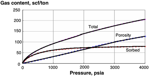
Figure 7.3 Gas content in free and absorbed gas. From Frantz et al., 2005.
Figure 7.3 shows how total gas content can be much higher than free gas, which is the only one accounted for in a conventional reservoir. This change in gas content with pressure in the Barnett shale indicates that for low-permeability formations, pseudo-radial flow can take over 100 years to be established. Thus, most gas flow in the reservoir is a linear flow from the near fracture area toward the nearest fracture face. This graph shows the complication in estimating performance of unconventional gas reservoir.
Similarly, pressure and drainage in CBM reservoirs are different from conventional reservoirs. Methane drainage is the process of removing the methane gas contained in the coal seam and surrounding strata through pipelines. Control techniques for use in coal mines can be divided into three categories: (1) dilution ventilation, (2) blocking or diverting gas flow in the coalbed by means of seals, and (3) removing relatively pure or diluted methane through boreholes. The drained gas is mostly methane. However, the main mechanism of methane production is dewatering or water production in contrast to conventional oil or gas production, which relies on depressurizing the pore pressure. There are four main methods used for methane recovery:
• the vertical degas;
• vertical gob degas system;
• horizontal borehole degas system; and
• the cross-measure borehole system.
Overall, unconventional gas wells show decline depicted in Figure 7.4. This figure shows how pressure decline can be arrested with hydraulic fracturing. However, this is an optimistic scenario. In previous chapters, it has been pointed out that the success of hydraulic fracturing depends on specifics of a reservoir. Note that hydraulically fractured tight gas wells do not decline exponentially. In almost all cases, they will decline hyperbolically.
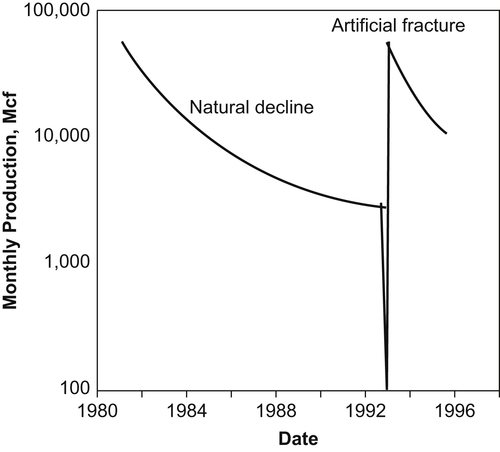
Figure 7.4 Typical decline curve for a tight gas reservoir. Redrawn from Holditch, 2006.
Gas production can be analyzed using log–log plots of rate or dimensionless rate versus time or dimensionless time, plots of inverse of normalized rates versus square root of time (called square root plots), following material balance plots, dimensionless plots, rate derivative plots, rate integral plots, and rate integral derivative plots, among others. Anderson et al. (2010) point out that the first three are particularly well-suited for tight gas and shale gas production analyses.
If one plots square root plots, log–log rate (q) versus time (t) plots, and log–log plots of dimensionless rate (qD) versus dimensionless time (tD), the plots show the different flow regimes exhibited by the reservoir, while the square root plot indicates the size of the “stimulated reservoir volume” during linear flow. The dimensionless variables are as defined below:
qD=141.2qμkh(pi−pwf)
![]()
tD=0.0002637ktϕμctx2f.
![]()
μ = viscosity, cp
q = gas flow rate in reservoir, cu ft
k = the matrix permeability, mD
h = the reservoir thickness, ft
pi = the initial reservoir pressure, psia
pwf = the flowing bottomhole pressure, psia
t = time, h
ϕ = porosity as a fraction
ct = total compressibility, psi−1
xf = the fracture half-length, ft
All decline curve analysis techniques depend on solving the diffusivity equation, which is given in the following form in the case of anisotropic reservoir (Eqn (7.4)):
kx∂2p∂x2+ky∂2p∂y2+kz∂2p∂z2=ϕμct∂p∂t
![]() (7.4)
(7.4)
All decline curve analyses involve solution of the diffusivity equation with analytical models. Because the equation is inherently nonlinear, simplifications must be made in order to solve the equation analytically. Most common assumption involves a semi-infinite domain. Others have used infinite extent of the reservoir. Yet, others have also used closed rectangular system in order to solve the governing equation. The infinite model has no-flow boundaries at the top and the bottom. The semi-infinite reservoir model has three no-flow boundaries (top, bottom, and left). The closed reservoir model has all four no-flow boundaries. Placing the well within the boundary poses additional constraints due to the imposition of a boundary condition. Typically, unconventional reservoirs are modeled with horizontal wells. Such wells are simulated as a line drive. This modeling makes the additional assumption that there is no pressure drop along the wellbore. For most cases, of gas flow, this is a reasonable assumption. Ozkan et al. (1987) solved the equation with Laplace transform, using infinite domain for a horizontal well and closed rectangular box for the reservoir. Results are compared with numerical simulation results in Figure 7.5.
The presence of natural fracture is inherent to unconventional gas. As such, any modeling should include natural fractures. While it has been recognized that natural fractures should produce oscillatory surge in oil/gas production, no one has attempted to model natural fractures that would produce such a production regime. Figure 7.6 shows how a dual porosity, dual permeability regime would produce gas surges in periodic fashion. Such behavior can be explained with interactions between capillary flow, storage, and fracture flow. Figure 7.7 shows experimental results conducted by Delgadillo-Velazquez et al., (2008). Such behavior occurs because of difference in shear rates and capillary intrusion, which is typical in a porous medium with fractures. In addition, fluid rheology plays a role, which adds further complication in modeling (Hossain and Islam, 2008).
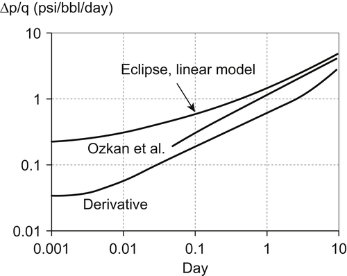
Figure 7.5 Comparison of linear model (homogeneous, zero skin, closed) with Fekete, ECLIPSE, and Ozkan Laplace solution. Redrawn from Bello, 2009.
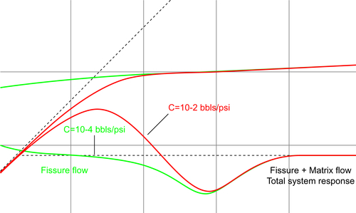
Figure 7.6 Pressure response in a fracture formation.
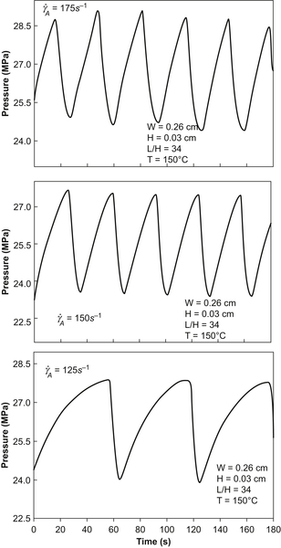
Figure 7.7 Typical pressure oscillations in slit flow at 150 °C. From Delgadillo-Velazquez et al., 2008.
In order to model shale gas and tight gas reservoirs, various analytical and semianalytical solutions have been proposed. Gringarten (Gringarten and Ramey, 1973; Gringarten, 1984) developed some of the early analytical models for flow through domains involving a single vertical fracture and a single horizontal fracture. A more complex series of semianalytical models for single vertical fractures were developed much later (Blasingame and Poe Jr., 1993). Prior to the development of models for multiple-fracture horizontal wells (Medeiros et al., 2006), it was common practice to represent these multiple fractures with an equivalent single fracture. In all these, however, the assumptions are the same and ultimate results are not improved from scientific perspective.
Several other analytical and semianalytical models have been developed since Bello and Wattenbarger (2008); Mattar (2008); Anderson et al., (2010). Although these models are much faster than numerical simulators, they generally cannot accurately handle the very high nonlinear aspects of shale gas and tight gas reservoirs because these analytical solutions address the nonlinearity in gas viscosity, compressibility, and compressibility factor with the use of pseudo-pressures (an integral function of pressure, viscosity, and compressibility factor) rather than solving the real gas flow equation. Other limitations include the difficulty in accurately capturing gas desorption from the matrix, multiphase flow, unconsolidation, and several nonideal and complex fracture networks (Houze et al., 2010).
The limitations of the analytical and semianalytical models have led to the use of numerical reservoir simulators to study the reservoir performance of these unconventional gas reservoirs. Miller et al., (2010) and Jayakumar et al., (2011) showed the application of numerical simulation to history-matching and forecasting production from two different shale gas fields, while Cipolla et al., (2009), Freeman et al., (2009), and Moridis et al. (2010) conducted numerical sensitivity studies to identify the most important mechanisms and factors that affect shale gas reservoir performance. These numerical studies show that the characteristics and properties of the fractured system play a dominant role in the reservoir performance. Hence, significant effort needs to be invested in the characterization and representation of the fractured system.
Carvalho and Rosa (1988) presented solutions for an infinite conductivity horizontal well in a semi-infinite reservoir. The reservoir was considered to be homogeneous and isotropic. The horizontal well is modeled as a line source. The solutions for the homogeneous case were then extended to the dual porosity case by substituting s∗f(s) for s in Laplace space for the pressure derivative (homogeneous). Wellbore storage and skin are incorporated into their model using Laplace space.
Aguilera and Ng (1989) presented analytical equations for pressure transient analysis. Their model is a horizontal well in a semi-infinite, anisotropic, naturally fractured reservoir. Transient and pseudo-steady state interporosity flow is considered. Six flow periods are identified—first radial flow (at early times, from fractures), transition period, second radial flow in vertical plane, first linear flow, pseudo-radial flow, and late linear flow—with expressions for determining the skin provided.
Ng and Aguilera (1989) presented analytical solutions using a line source and then compute pressure drop on a point away from the well axis to account for the radius of the actual well. A method for determining the numerical Laplace transform is presented. This method was then used to compute the dual porosity response (pseudo-steady state).
Thompson et al. (1991) presented an algorithm for computing horizontal well response in a bounded dual porosity reservoir. Their model is a horizontal well in a closed rectangular reservoir. Their procedure involves converting a known analytic solution to Laplace space numerically point by point and then inverting using the Stehfest algorithm. This is similar to the procedure presented by Ohaeri and Vo (1991) who use a numerical Laplace space algorithm, but present alternative equations determined by parameter ranges that result in computational efficiency.
Du and Stewart (1992) described situations that can yield linear flow behavior: a multilayered reservoir (one layer has a very high permeability relative to the other); naturally fractured reservoir (flow from matrix into horizontal well intersecting fractures); and areal anisotropy (vertical fractures aligned predominantly in one direction). Their model is a horizontal well in a homogeneous, infinite acting reservoir. Three flow regimes are identified: radial vertical flow, linear flow opposite to completed section, and pseudo-radial flow at late time. A bilinear flow behavior was also identified.
7.2.1.3. Statistical Method
In this method, the past performance of numerous reservoirs is statistically accounted for to derive the empirical correlations, which are used for future predictions. It may be described as a “formal extension of the analogical method.” The statistical methods have the following assumptions.
• Reservoir properties are within the limit of the database.
• Reservoir symmetry exists.
• Ultimate recovery is independent of the rate of production.
In addition, Islam et al. (2014) recently pointed out a more subtle, yet far more important shortcoming of the statistical methods. Practically, all statistical methods assume that two or more objects based on a limited number of tangible expressions make it legitimate to comment on the underlying science. It is equivalent to stating that if effects show a reasonable correlation, the causes can also be correlated. As Zatzman and Islam (2006) pointed out, this poses a serious problem as, in absence of time–space correlation (pathway rather than end result), anything can be correlated with anything, making the whole process of scientific investigation spurious. They make their point by showing the correlation between global warming (increases) with a decrease in the number of pirates (Figure 7.8). The absurdity of the statistical process becomes evident by drawing this analogy. Shapiro et al. (2006) pointed out another severe limitation of the statistical method. Even though they commented on the polling techniques used in various surveys, their comments are equally applicable in any statistical modeling. They wrote: “Frequently, opinion polls generalize their results to a U.S. population of 300 million or a Canadian population of 32 million on the basis of what 1,000 or 1,500 ‘randomly selected’ people are recorded to have said or answered. In the absence of any further information to the contrary, the underlying theory of mathematical statistics and random variability assumes that the individual selected ‘perfectly’ randomly is no more nor less likely to have any one opinion over any other. How perfect the randomness may be determined from the ‘confidence’ level attached to a survey, expressed in the phrase that describes the margin of error of the poll sample lying plus or minus some low single-digit percentage ‘nineteen times out of twenty’, i.e., a confidence level of 0.95. Clearly, however, assuming in the absence of any knowledge otherwise a certain state of affairs to be the case, viz., that the sample is random and no one opinion is more likely than any other, seems more useful for projecting horoscopes than scientifically assessing public opinion.”
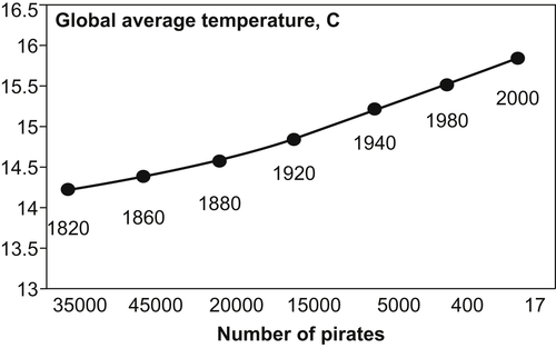
Figure 7.8 Using statistical data to develop a theoretical correlation that can make an aphenomenal model appealing, depending on which conclusion would appeal to the audience.
Probability experiments have been some of the least controversial techniques for determining future course of actions. However, recently it has come to light that such assertion is not warranted (see Islam et al., 2014a, 2014b, 2015).
Consider the following example. If you know there are three white balls and two black balls in a bag, what is the probability of finding a white ball if you attempt to withdraw a ball from the bag? Of course, it is three out of five. The same way, probability of drawing a black ball is two out of five. However, if one asks what is the probability of drawing a pink ball, what would be the answer? If the answer is “zero,” it would violate the quantum physics principle that nothing is absolutely improbable, except the existence of a creator. What other principle does a zero probability violate?
Scientific answer is the probability of finding a pink ball is zero unless someone truthful confirms that the premise that only black and white balls exist in the bag is untrue or the actual content of the bag is unknown as a function of time.
Say after a certain time, a draw was made and a pink ball was drawn at the first trial. This observation shows that the premise that there were only black and white balls present in the bag is untrue. This confusion could be avoided if there were some room to account for the time function or history of the bag in question in probability theories. There is none. Probability theory by definition assumes steady state in all matters and does not include the time function. How would it look like if the time function were included?
Consider the following example. A draw of head and tail is made repeatedly. Probability theory assumes that if the draw is made infinite number of times, the ratio of head and tail would be 1. In essence, it introduces a time function that is self-imposed and there is no way to verify the validity of this time function. It is because infinity is not achievable in a physical experiment. In Figure 7.9, an actual observation of coin toss is plotted. The y-axis represents the ratio of head and tail, while the x-axis represents the number of coin toss. It is clear that as the number of coin toss increases, the most probable occurrence of head or tail settles around a ratio of 2. This is in sharp contrast to the conventional notion of 1.
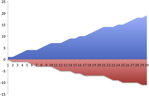
Figure 7.9 Number of coin toss vs head (+sign) and tail (−sign) in an actual experiment.
Figure 7.10 also shows how at no time the distribution of head and tail follows the 1:1 rule. As the number of coin toss is increased, the distribution actually diverges and settles toward a value outside of 1:1 distribution. If the number of coin toss is increased, the conventional approach says the number of head and tail ratio would be closer to 1. It means, if this number is increased to infinity, the ratio would converge to 1.
This simple experiment goes to demonstrate how a fundamentally flawed paradigm is introduced by selecting a probability model.
Theoretically, if the premise of “steady state” probability is removed, data gathered on certain population can be helpful only if the data volume and time involved are representative. In engineering, the notion of representative elementary volume (REV) is well known. Here, we introduce the notion of representative elemental time, which is in essence characteristic frequency of a process. For every entity, there is a characteristic frequency, which itself is a function of time. This notion has been discussed by Islam et al. (2014a). Figure 7.11 represents the relationship between characteristic value and number of trials. Similar figure applies to the number of subjects in a survey.
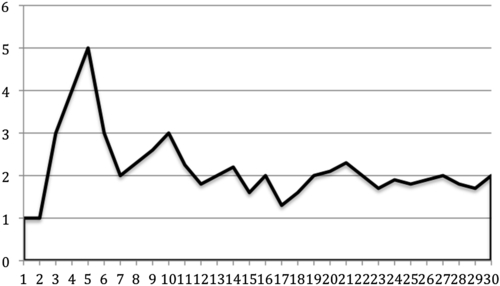
Figure 7.10 As the number of coin toss is increased, the head and tail toss ratio converges toward 2 and not 1.
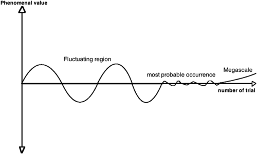
Figure 7.11 Number of trials is likely to yield different sets of phenomenal values that apply to different entities.
One side effect of statistical rules is the so-called Simpson's paradox. This paradox states that for continuous data, a positive trend appears for two separate groups (blue and red) and a negative trend (black, dashed) appears when the data are combined (Figure 7.12). In probability and statistics, Simpson's paradox, or the Yule–Simpson effect, is a paradox in which a trend that appears in different groups of data disappears when these groups are combined, and the reverse trend appears for the aggregate data. This result is often encountered in social-science and medical-science statistics. Islam et al. (2010a) discussed this phenomenon as something that is embedded in Newtonian calculus that allows taking the infinitely small differential and turning that into any desired integrated value, while giving the impression that a scientific process has been followed. Furthermore, Khan and Islam (2012) showed that true trend line should contain all known parameters. The Simpson's paradox can be avoided by including full historical data, followed by scientifically true processing (Islam et al., 2014a; Pearl, 2009).
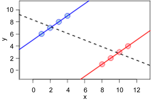
Figure 7.12 Simpson's paradox highlights the problem of targeted statistics.
The above difficulty with statistical processing of data was brought into highlight through the publication of the following correlation between number of pirates versus global temperature with the slogan: Join piracy, save the planet.
Similar paradox arises from the so-called ecological fallacies. It is best described in Wikipedia with the following examples:
Assume that at the individual level, being Protestant impacts negatively one's tendency to commit suicide but the probability that one's neighbor commits suicide increases one's tendency to become Protestant. Then, even if at the individual level there is negative correlation between suicidal tendencies and Protestantism, there can be a positive correlation at the aggregate level.
Similarly, even if at the individual level, wealth is positively correlated to tendency to vote Republican, we observe that wealthier states tend to vote Democrat. For example, in 2004, the Republican candidate, George W. Bush, won the fifteen poorest states, and the Democratic candidate, John Kerry, won 9 of the 11 wealthiest states. Yet 62% of voters with annual incomes over $200,000 voted for Bush, but only 36% of voters with annual incomes of $15,000 or less voted for Bush.
The prosecutor's fallacy is a fallacy of statistical reasoning, typically used by the prosecution to argue for the guilt of a defendant during a criminal trial. In its crudest form, it involves the assertion that the probability of defendant to be guilty is 90% because the perpetrator and the defendant are known to be sharing the blood type that has a probability of 10% in the general population. It is purported that a DNA match is not a fallacy because the probability of match is much greater. However, this is also an example of how New Science has refined techniques in favor of opacity instead of transparency. The use of DNA as the only match has the gravest risk of “creating” evidence in case there is no other evidence. This is rarely talked about. Such mind-set has promoted prosecution tactics that allowed torture as a means of extracting “evidence.” In a broader sense, it has also allowed notorious conclusions, such as the nonconsideration of junk DNA, asserting probability of Big Bang as 97%, probability of life as “reasonable,” probability of “intelligent life” as even “more reasonable,” and others. All of them suffer from the fundamental basis that a “fact is not a matter of probability.” For instance, the proclamation that orangutan is linked to humans because the DNA match is the greatest (Derbyshire, 2011), What can be said when a greater match of some other component of genome is found with certain plants?
7.2.1.4. Finite Difference Methods
Finite difference calculus is a mathematical technique, which is used to approximate values of functions and their derivatives at discrete points, where they are not known. The history of differential calculus dates back to the time of Leibnitz and Newton. In this concept, the derivative of a continuous function is related to the function itself. The Newton's formula is the core of differential calculus and suffers from the approximation that magnitude and direction change independently of one another. There is no problem in having separate derivatives for each component of the vector or in superimposing their effects separately and regardless of order. That is what mathematicians mean when they describe or discuss Newton's derivative being used as a “linear operator.” Following this, comes Newton's difference quotient formula. When the value of a function is inadequate to solve a problem, the rate at which the function changes, sometimes, becomes useful. Therefore, the derivatives are also important in reservoir simulation. In Newton's difference quotient formula, the derivative of a continuous function is obtained. This method relies implicitly on the notion of approximating instantaneous moments of curvature, or infinitely small segments, by means of straight lines. This alone should have tipped everyone off that his derivative is a linear operator precisely because, and to the extent that, it examines change over time (or distance) within an already established function (Islam et al., 2010). This function is applicable to an infinitely small domain, making it nonexistent. When integration is performed, however, this nonexistent domain is assumed to be extended to finite and realistic domain, making the entire process questionable.
The finite difference methods are extensively applied in petroleum industry to simulate the fluid flow inside the porous medium. The following assumptions are inherent to the finite difference method.
1. The relationship between derivative and the finite difference operators, e.g., forward, backward, and central difference operators, is established through the Taylor series expansion. The Taylor series expansion is the base element in providing the differential form of a function. It converts a function into polynomial of infinite order. This provides an approximate description of a function by considering a finite number of terms and ignoring the higher order parts. In other words, it assumes that a relationship between the operators of discrete points and the operators of the continuous functions is acceptable.
2. The relationship involves truncation of the Taylor series of the unknown variables after few terms. Such truncation leads to accumulation of error. Mathematically, it can be shown that most of the error occurs in the lowest order terms.
a. The forward and the backward difference approximations are the first order approximations to the first derivative.
b. Although the approximation to the second derivative by the central difference operator increases accuracy because of a second order approximation, it still suffers from the truncation problem.
c. As the spacing size reduces, the truncation error approaches to zero more rapidly. Therefore, a higher order approximation will eliminate the need of same number of measurements or discrete points. It might maintain the same level of accuracy; however, less information at discrete points might be risky as well.
3. The solutions of the finite difference equations are obtained only at the discrete points. These discrete points are defined either according to block-centered or point-distributed grid system. However, the boundary condition, to be specific, the constant pressure boundary, may appear important in selecting the grid system with inherent restrictions and higher order approximations.
4. The solutions obtained for grid points are in contrast to the solutions of the continuous equations.
5. In the finite difference scheme, the local truncation error or the local discretization error is not readily quantifiable because the calculation involves both continuous and discrete forms. Such difficulty can be overcome when the mesh size or the time step or both are decreased leading to minimization in local truncation error. However, at the same time the computational operation increases, which eventually increases the round-off error.
Zatzman et al., 2007 identified the most significant contribution of Newton in mathematics: the famous definition of the derivative as the limit of a difference quotient involving changes in space or in time as small as anyone might like, but not zero, viz.
ddtf(t)=limΔt→0f(t+Δt)−f(t)Δt
![]() (7.5)
(7.5)
Without regards to further conditions being defined as to when and where differentiation would produce a meaningful result, it was entirely possible to arrive at “derivatives” that would generate values in the range of a function at points of the domain where the function was not defined or did not exist. Indeed, it took another century following Newton's death before mathematicians would work out the conditions—especially the requirements for continuity of the function to be differentiated within the domain of values—in which its derivative (the name given to the ratio quotient generated by the limit formula) could be applied and yield reliable results. Kline (1972) detailed the problems involving this breakthrough formulation of Newton. However, no one in the past did propose an alternative to this differential formulation, at least not explicitly. The following figure (Figure 7.13) illustrates this difficulty.
In this figure, economic index (it may be one of many indicators) is plotted as a function of time. In nature, all functions are very similar. They do have local trends as well as global trends (in time). One can imagine how the slope of this graph on a very small time frame would be quite arbitrary, and how devastating it would be to take that slope to a long term. One can easily show that the trend emerging from Newton's differential quotient would be diametrically opposite to the real trend. Zatzman and Islam (2007b) provided a basis for determining real gradient, rather than local gradient that emerges from Newton's differential quotient. In that formulation, it is shown that the actual value of Δt over which the reliable gradient has to be observed needs to be several times greater than the characteristic time of a system. The notion of REV, as first promoted by Bear (1972), is useful in determining a reasonable value for this characteristic time. The second principle is that at no time Δt be allowed to approach 0 (Newton's approximation), even when the characteristic value is very small (e.g., phenomena at nanoscale). With the engineering approach, it turns out such approximation is not necessary (Abou-Kassem, 2007) because this approach bypasses the recasting of governing equations into Taylor series expansion, instead relying on directly transforming governing equations into a set of algebraic equations. In fact, by setting up the algebraic equations directly, one can make the process simple and yet maintain accuracy (Mustafiz et al., 2008). Finally, initial analysis should involve the extension Δt to ∞ in order to determine the direction, which is related to sustainability of a process (Zatzman et al., 2008).
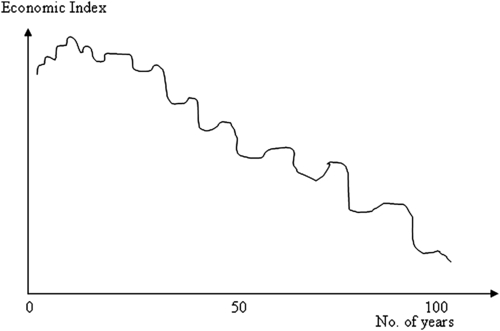
Figure 7.13 Economic well-being is known to fluctuate with time.
Figure 7.14 shows how formulation with the engineering approach ends up with the same linear algebraic equations if the inside steps are avoided. Even though the engineering approach was known for decades (known as the control volume approach), no one identified in the past the advantage of removing in-between steps.
7.2.1.4.1. Darcy's Law
Because practically all reservoir simulation studies involve the use of Darcy's law, it is important to understand the assumptions behind this momentum balance equation. The following assumptions are inherent to Darcy's law and its extension.
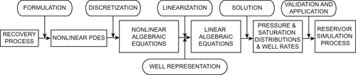
Figure 7.14 Major steps to develop reservoir simulators. Redrawn from Abou-Kassem et al., 2006.
• The fluid is homogenous, single phase and Newtonian.
• No chemical reaction takes place between the fluid and the porous medium.
• Laminar flow condition prevails.
• Permeability is a property of the porous medium, which is independent of pressure, temperature, and the flowing fluid.
• There is no slippage effect, e.g., Klinkenberg phenomenon.
• There is no electrokinetic effect.
Clearly, Darcy's law does not apply to unconventional reservoirs. The matrix permeability is too low, which means dispersive term should be included. The inclusion of Brinkman term can solve this problem. As for the fracture, inertial forces are high, thereby making Darcy's law invalid. This is particularly important for gas reservoirs, for which Forchheimer equation should be used. This aspect is discussed later in this chapter.
7.3. Recent Advances in Reservoir Simulation
The recent advances in reservoir simulation may be viewed as:
• speed and accuracy,
• new fluid flow equations,
• coupled fluid flow and geomechanical stress model, and
• fluid flow modeling under thermal stress.
7.3.1. Speed and Accuracy
The need for new equations in oil reservoirs arises mainly for fractured reservoirs as they constitute the largest departure from Darcy's flow behavior. Advances have been made in many fronts. As the speed of computers increased following Moore's law (doubling every 12–18 months), the memory also increased. For reservoir simulation studies, this translated into the use of higher accuracy through inclusion of higher order terms in Taylor series approximation as well as great number of grid blocks, reaching as many as billion blocks. The greatest difficulty in this advancement is that the quality of input data did not improve at par with the speed and memory of the computers. As Figure 7.15 shows that the data gap remains possibly the biggest challenge in describing a reservoir. Note that the inclusion of large number of grid blocks makes the prediction more arbitrary than that predicted by fewer blocks, if the number of input data points is not increased proportionately. The problem is particularly acute when fractured formation is being modeled. The problem of reservoir cores being smaller than the REV is a difficult one, which is more accentuated for fractured formations that have a higher REV. For fractured formations, one is left with a narrow band of grid blocks, beyond which solutions are either meaningless (large grid blocks) or unstable (too small grid blocks).
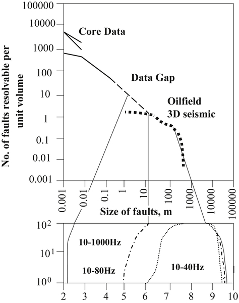
Figure 7.15 Data gap in geophysical modeling. After Islam, 2001.
The problem is particularly intense for unconventional reservoirs for which few logging techniques produce meaningful results and core data are mostly nonrepresentative. The reservoir characterization technique proposed in Chapter 5 outlines a way out of this dilemma. With proper reservoir characterization, the data gap can be filled with filtered data.
7.3.2. New Fluid Flow Equations
A porous medium can be defined as a multiphase material body (solid phase represented by solid grains of rock and void space represented by the pores between solid grains) characterized by two main features: that a REV can be determined for it, such that no matter where it is placed within a domain occupied by the porous medium; and it will always contain both a persistent solid phase and a void space. The size of the REV is such that parameters that represent the distributions of the void space and the solid matrix within it are statistically meaningful.
Theoretically, fluid flow in porous medium is understood as the flow of liquid or gas or both in a medium filled with small solid grains packed in homogeneous manner. The concept of heterogeneous porous medium is then introduced to indicate change in properties (mainly porosity and permeability) within that same solid grains packed system. An average estimation of properties in that system is an obvious solution, and the case is still simple.
Incorporating fluid flow model with a dynamic rock model during the depletion process with a satisfactory degree of accuracy is still difficult to attain from currently used reservoir simulators. Most conventional reservoir simulators do not couple stress changes and rock deformations with reservoir pressure during the course of production and do not include the effect of change of reservoir temperature during thermal or steam injection recoveries. The physical impact of these geomechanical aspects of reservoir behavior is neither trivial nor negligible. Pore reduction and/or pore collapse leads to abrupt compaction of reservoir rock, which in turn causes miscalculations of ultimate recoveries, damage to permeability, and reduction to flow rates and subsidence at the ground and well casing's damage. In addition, there are many reported environmental impacts due to the withdrawal of fluids from underground reservoirs. Using only Darcy's law to describe hydrocarbon fluid behavior in petroleum reservoirs when high gas flow rate is expected or when encountered highly fractured reservoir is totally misleading. Nguyen (1986) has showed that using standard Darcy flow analysis in some circumstances can overpredict the productivity by as much as 100%.
Fracture can be defined as any discontinuity in a solid material. In geological terms, a fracture is any planar or curvy planar discontinuity that has formed as a result of a process of brittle deformation in the earth's crust. Planes of weakness in rock respond to changing stresses in the earth's crust by fracturing in one or more different ways depending on the direction of the maximum stress and the rock type. A fracture can be said to consist of two rock surfaces, with irregular shapes, which are more or less in contact with each other. The volume between the surfaces is the fracture void. The fracture void geometry is related in various ways to several fracture properties. Fluid movement in a fractured rock depends on discontinuities, at a variety of scales ranging from microcracks to faults (in length and width). Fundamentally, describing flow through fractured rock involves describing physical attributes of the fractures: fracture spacing, fracture area, fracture aperture, and fracture orientation and whether these parameters allow percolation of fluid through the rock mass. Fracture parameters also influence the anisotropy and heterogeneity of flow through fractured rock. Thus the conductivity of a rock mass depends on the entire network within the particular rock mass and is thus governed by the connectivity of the network and the conductivity of the single fractures. The total conductivity of a rock mass depends also on the contribution of matrix conductivity at the same time.
A fractured porous medium is defined as a portion of space in which the void space is composed of two parts: an interconnected network of fractures and blocks of porous medium, and the entire space within the medium occupied by one or more fluids. Such a domain can be treated as a single continuum, provided an appropriate REV can be found for it.
The fundamental question to be answered in modeling fracture flow is the validity of the governing equations used. The conventional approach involves the use of dual porosity, dual permeability models for simulating flow through fractures. Choi et al. (1997) demonstrated that the conventional use of Darcy's law in both fracture and matrix of the fractured system is not adequate. Instead, they proposed the use of the Forchheimer model in the fracture while maintaining Darcy's law in the matrix. Their work, however, was limited to single-phase flow. In future, the present status of this work can be extended to a multiphase system. It is anticipated that gas reservoirs will be suitable candidates for using Forchheimer extension of the momentum balance equation, rather than the conventional Darcy's law. Similar to what was done for the liquid system (Cheema and Islam, 1995), opportunities exist in conducting experiments with gas as well as multiphase fluids in order to validate the numerical models. It may be noted that in recent years several dual porosity, dual permeability models have been proposed based on experimental observations (Tidwell and Robert, 1995; Saghir et al., 2001).
For unconventional reservoirs, Brinkman equation has to be used in the matrix. It is the case because of the low permeability of the matrix. This will be detailed in a later section of this chapter.
7.3.3. Coupled Fluid Flow and Geomechanical Stress Model
Coupling different flow equations has always been a challenge in reservoir simulators. In this context, Pedrosa et al. (1986) introduced the framework of hybrid grid modeling. Even though this work was related to coupling cylindrical and Cartesian grid blocks, it was used as a basis for coupling various fluid flow models (Islam and Chakma, 1990). Coupling flow equations in order to describe fluid flow in a setting, for which both pipe flow and porous media flow prevail, continues to be a challenge (Islam et al., 2010). For unconventional gas, horizontal wells are of great importance. Even though it is commonly perceived that pressure drop in the horizontal well within a gas reservoir is negligible, this is not the case in many scenarios, particularly the ones involving multiphase flow. For example, one can cite coalbed methane, condensate, and even some tight gas formations with oil flow.
Geomechanical stresses are very important in production schemes. However, due to strong seepage flow, disintegration of formation occurs and sand is carried toward the well opening. The most common practice to prevent accumulation as followed by the industry is to take filter measures, such as liners and gravel packs. Generally, such measures are very expensive to use and often, due to plugging of the liners, the cost increases to maintain the same level of production. In recent years, there have been studies in various categories of well completion including modeling of coupled fluid flow and mechanical deformation of medium (Vaziri et al., 2003). Vaziri et al. (2003) used a finite element analysis developing a modified form of the Mohr–Coulomb failure envelope to simulate both tensile and shear-induced failure around deep wellbores in oil and gas reservoirs. The coupled model was useful in predicting the onset and quantity of sanding. Nouri et al. (2006) highlighted the experimental part of it in addition to a numerical analysis and measured the severity of sanding in terms of rate and duration. It should be noted that these studies (Nouri et al., 2002; Vaziri et al., 2003 and Nouri et al., 2006) took into account the elastoplastic stress–strain relationship with strain softening to capture sand production in a more realistic manner. Although, at present these studies lack validation with field data, they offer significant insight into the mechanism of sanding and have potential in smart designing of well completions and operational conditions.
Settari et al. (2006) applied numerical techniques to calculate subsidence induced by gas production in the North Adriatic. Due to the complexity of the reservoir and compaction mechanisms, Settari et al. (2006) took a combined approach of reservoir and geomechanical simulators in modeling subsidence. As well, an extensive validation of the modeling techniques was undertaken, including the level of coupling between the fluid flow and geomechanical solution. The researchers found that a fully coupled solution had an impact only on the aquifer area and an explicitly coupled technique was good enough to give accurate results. On grid issues, the preferred approach was to use compatible grids in the reservoir domain and to extend that mesh to geomechanical modeling. However, it was also noted that the grids generated for reservoir simulation are often not suitable for coupled models and require modification.
In fields, on several instances, subsidence delay has been noticed and related to overconsolidation, which is also termed as the threshold effect (Merle et al., 1976; Hettema et al., 2002). Settari et al. (2006) used the numerical modeling techniques to explore the effects of small levels of overconsolidation in one of their studied fields on the onset of subsidence and the areal extent of the resulting subsidence bowl. The same framework that Settari et al. (2006) used can be introduced in coupling the multiphase, compositional simulator and the geomechanical simulator in future.
7.3.4. Fluid Flow Modeling under Thermal Stress
The temperature changes in the rock can induce thermoelastic stresses (Hojka et al., 1993), which can either create new fractures or can alter the shapes of existing fractures, changing the nature of primary mode of production. It can be noted that the thermal stress occurs as a result of the difference in temperature between injected and reservoir fluids or due to the Joule–Thomson effect. However, in the study with unconsolidated sand, the thermal stresses are reported to be negligible in comparison to the mechanical stresses (Chalaturnyk et al., 1995). Similar trend is noticeable in the work by Chen et al. (1995), which also ignored the effect of thermal stresses, even though a simultaneous modeling of fluid flow and geomechanics is proposed.
Most of the past research has been focused only on thermal recovery of heavy oil. Modeling subsidence under thermal recovery technique (Tortike and Farouq Ali, 1987) was one of the early attempts that considered both thermal and mechanical stresses in their formulation. There are only few investigations that attempted to capture the onset and propagation of fractures under thermal stress. Zekri et al. (2006) investigated the effects of thermal shock on fractured core permeability of carbonate formations of UAE reservoirs by conducting a series of experiments. Also, the stress–strain relationship due to thermal shocks was noted. Apart from experimental observations, there is also the scope to perform numerical simulations to determine the impact of thermal stress in various categories, such as water injection, gas injection/production, etc.
7.3.5. Challenges of Modeling Unconventional Gas Reservoirs
Most modeling approaches in unconventional gas reservoirs involve flow equations that are not valid for unconventional cases. In addition, complexities arise from complex geometry that prevails in unconventional reservoirs. For instance, the traditional approach of modeling fractured shale gas reservoirs with regular Cartesian grids could be limited in that it cannot efficiently represent complex geologies, including nonplanar and nonorthogonal fractures, and cannot adequately capture the elliptical flow geometries expected around the fracture tips in such fractured reservoirs. It also suffers from the fact that the number of grids can easily grow into millions because of the inability to change the orientation and shape of the grids away from the fracture tips, thus requiring extremely fine discretization in an attempt to describe all possible configurations. This problem is also aggravated by the large number (up to 60) of hydraulic fractures in a clustered fracture system (Jayakumar et al., 2011). The problem is more intense for natural fractures.
Moridis et al. (2010) identified the distinct fracture systems present in producing shale gas and tight gas reservoirs. Figure 7.16 shows a graphical illustration of the following four fracture systems.
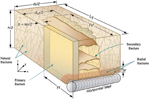
Figure 7.16 Identification of the four fractured systems. From Moridis et al., 2010.
• Primary or hydraulic fractures: These are fractures that are typically created by injecting hydrofracturing fluids (with or without proppants) into the formation. Proppants provide high-permeability flow paths that allow gas to flow more easily from the formation matrix into the well. Artificial fractures are predominantly orthogonal to natural fractures.
• Secondary fractures: These fractures are termed “secondary” because they are induced as a result of changes in the geomechanical status of a rock when the primary fractures are being created. Microseismic fracture mappings suggest that they generally intersect the primary fractures, either orthogonally or at an angle. Most prior studies assumed ideal configurations with orthogonal and planar fracture intersections so as to simplify the gridding; but in this work, we have developed an unstructured mesh maker that facilitates the gridding of nonorthogonal, nonplanar, and other nonideal fracture geometries.
• Natural fractures: As the name implies, these fractures are native to the formation in the original state, prior to any well completion or fracturing process. These fractures are result of faults that are part of broader tectonic of the reservoir.
• Radial fractures: These are fractures that are created as a result of stress releases in the immediate neighborhood of the horizontal well. This is integral part of the invasion due to drilling.
Efforts have been made in order to simplify the above geometry in a tractable form. Houze et al. (2010) recognized the importance of explicitly gridding secondary fractures so as to quantify the interaction between primary and secondary networks as distinct systems, using either a regular orthogonal pattern or a more random and complex system. In this work, we have identified two classes of possible fracture geometries/orientations:
• Regular or ideal fractures: These are idealized fracture geometries, which are usually planar and orthogonal. A perfectly planar (or orthogonal fracture) is the idealized geometry used in numerical studies using Cartesian grids. Figure 7.17a gives an illustration of this fracture geometry.
• Irregular or nonideal fractures: These are the kinds of fracture geometries we are likely to encounter in real life. They could be nonorthogonal, meaning that the fractures intersect either the well (for primary fractures) or primary fractures (for secondary fractures) at angles other than 90°, and they could be complex, meaning that the fractures are not restricted to a flat, nonundulating plane. Figures 7.17b and 7.17c give a diagrammatic illustration of two such scenarios.
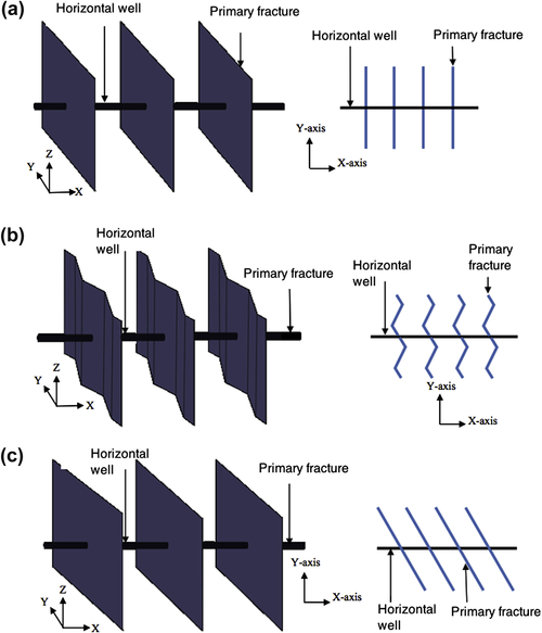
Figure 7.17 Simplification of fracture geometry.
Olorode (2011) reported modeling using nonorthogonal fractures (Figure 7.18). Figure 7.18 shows an almost identical rate profile for the nonplanar and nonorthogonal fracture systems at an angle of 60° to the horizontal. The fracture interference in these two cases becomes evident at the same time with the planar case that has a fracture half-length equal to the apparent length, la. The nonorthogonal fracture case with θ = 30° exhibits fracture interference earlier than the other cases, and this can be attributed to the fact that the apparent fracture half-length, la, is smaller in comparison to the other nonideal cases. The cumulative production plot shows that the nonideal fractured systems have lower production than the planar cases with the same fracture half-length. This implies that to the extent possible, fractures should be designed such that their angle of inclination with the horizontal well should be as close to 90° as possible. This can be achieved by ensuring that the horizontal well is drilled in the direction of the minimum principal stress, as fractures usually propagate perpendicularly to the direction of the minimum principal stress.
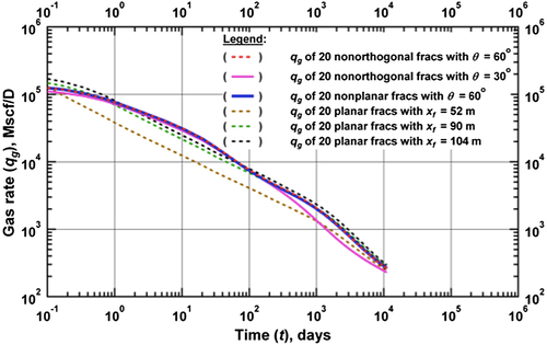
Figure 7.18 Flow profiles for nonplanar and nonorthogonal fractures. From Olorode, 2011.
Other challenges in modeling unconventional reservoirs lie within describing fracture flow and considering interactions between matrix and fracture. The original fracture flow model was developed in 1963 by Warren and Root. It assumed that the matrix has no permeability and the porosity is distributed in fractures as well as the matrix. Kazemi (1968) used a slab matrix model with horizontal fractures and unsteady state matrix–fracture flow to represent single-phase flow in the fractured reservoir. This was the first extension of the Warren–Root model. The assumptions included homogeneous behavior and isotropic matrix and fracture properties. He further assumed that the well is centrally located in a bounded radial reservoir. A numerical reservoir simulator was used. It was concluded that the results were similar to that of Warren–Root model when applied to a drawdown test in which the boundaries have not been detected. Two parallel straight lines were obtained on a semilog plot. The first straight line may be obscured by wellbore storage effects and the second straight line may lead to overestimating ω when boundary effects have been detected.
De Swaan (1975) presented a model that approximates the matrix blocks by regular solids (slab and spheres) and utilizes heat flow theory to describe the pressure distribution. It was assumed that the pressure in the fractures around the matrix blocks is variable and the source term is described through a convolution term. Approximate line-source solutions for early and late time are presented. The late time solutions are similar to those for early time except that modified hydraulic diffusivity terms dependent on fracture and matrix properties are included. The results are two parallel lines representing the early and late time approximations. The late time solution matches Kazemi (1968) for the slab case. De Swaan's model does not properly represent the transition period.
Najurieta (1980) presented a transient model for analyzing pressure transient data based on De Swaan's theory. Two types of fractured reservoir were studied: stratum (slabs) and blocks (approximated by spheres). The model predicted results similar to Kazemi (1968).
Serra et al. (1982) present methods for analyzing pressure transient data. The slab model used is similar to De Swaan (1975) and Najurieta (1980). The model considers unsteady state matrix–fracture transfer and is for an infinite reservoir. Three flow regimes were identified. Flow regime 1 and 3 are the Warren and Root's 18 early and late time semilog lines. A new flow regime 2 was also identified with half the slope of the late time semilog line.
Chen et al. (1985) presented methods for analyzing drawdown and buildup data for a constant rate producing well centrally located in a closed radial reservoir. The slab model similar to De Swaan (1975) and Kazemi (1968) is used. Five flow regimes are presented. Flow regimes 1, 2, and 3 are associated with an infinite reservoir and are described in Serra et al. (1982). Flow regime 1 occurs when there is a transient only in the fracture system. Flow regime 2 occurs when the transient occurs in the matrix and fractures. Flow regime 3 is a combination of transient flow in the fractures and “pseudo-steady state” in the matrix. Pseudo-steady state in the matrix occurs when the no-flow boundary represented by the symmetry center line in the matrix affects the response. Two new flow regimes associated with a bounded reservoir are also presented. Flow regime 4 reflects unsteady linear flow in the matrix system and pseudo-steady state in the fractures. Flow Regime 5 occurs when the response is affected by all the boundaries (pseudo-steady state).
Streltsova (1982) applied a “gradient model” (transient matrix–fracture transfer flow) with slab-shaped matrix blocks to an infinite reservoir. The model predicted results differ from the Warren–Root model in early time but converge to similar values in late time. The model also predicted a linear transitional response on a semilog plot between the early and late time pressure responses, which has a slope equal to half that of the early and late time lines. This linear transitional response was also shown to differ from the S-shaped inflection predicted by the Warren–Root model.
Cinco Ley and Samaniego (1982) utilized models similar to De Swaan and Najurieta and presented solutions for slab and sphere matrix cases. They utilize new dimensionless variables—dimensionless matrix hydraulic diffusivity, and dimensionless fracture area. They describe three flow regimes observed on a semilog plot: fracture storage dominated flow, “matrix transient linear”-dominated flow, and a matrix pseudo-steady state flow. The “matrix transient linear”-dominated flow period is observed as a line with one-half the slopes of the other two lines. It should be noted that the “matrix transient linear” period yields a straight line on a semilog plot indicating radial flow and might be a misnomer. The fracture storage dominated flow is due to fluid expansion in the fractures. The “matrix transient linear” period is due to fluid expansion in the matrix. The matrix pseudo-steady state period occurs when the matrix is under pseudo-steady state flow and the reservoir pressure is dominated by the total storativity of the system (matrix + fractures). It was concluded that matrix geometry might be identified with their methods, provided the pressure data is smooth.
Lai et al. (1983) utilize one-sixth of a cube matrix geometry transient model to develop well test equations for finite and infinite cases including wellbore storage and skin. Their model was verified with a numerical simulator employing the multiple interacting continua method.
Ozkan et al. (1987) presented an analysis of flow regimes associated with flow of a well at constant pressure in a closed radial reservoir. The rectangular slab model similar to De Swaan and Kazemi is used. Five flow regimes are presented: Flow regimes 1, 2, and 3 are described in Serra et al. (1982). Two new regimes are presented: Flow regime 4 reflects unsteady linear flow in the matrix system and occurs when the outer boundary influences the well response and the matrix boundary has no influence. Flow regime 5 occurs when the response is affected by all the boundaries.
Houze et al. (1988) presented type curves for analysis of pressure transient response in an infinite naturally fractured reservoir with an infinite conductivity vertical fracture.
Stewart and Ascharsobbi (1988) presented an equation for interporosity skin, which can be introduced into the pseudo-steady state and transient models. It should be noted that all the transient models previously described were developed for the radial reservoir cases (infinite or bounded).
El-Banbi (1998) was the first to present transient dual porosity solutions for the linear reservoir case. New solutions were presented for a naturally fractured reservoir using a dual porosity, linear reservoir model. Solutions are presented for a combination of different inner (constant pressure, constant rate, with or without skin and wellbore storage) and outer boundary conditions (infinite, closed, constant pressure).
Kucuk and Sawyer (1979, 1980) presented a model for transient matrix–fracture transfer for the gas case. Previous work had been concerned mainly with modeling slightly compressible (liquid) flow. They considered cylindrical and spherical matrix blocks cases. They also incorporate the pseudo-pressure definitions for gases. Techniques for analyzing buildup data are also presented for shale gas reservoirs. Their model results plotted on a dimensionless basis matched Warren and Root (1963) and Kazemi (1968) for very large matrix blocks at early time but differ at later times. They also conclude from their tests that naturally fractured reservoirs do not always exhibit the Warren–Root behavior (two parallel lines).
Carlson and Mercer (1989) coupled Fick's law for diffusion within the matrix and desorption in their transient radial reservoir model for shale gas. This is the closest to Brinkman formulation that any fluid flow model came in terms of unconventional reservoir modeling. Modifications included use of the pressure-squared forms valid for gas at low pressures to linearize the diffusivity equation. They provide a Laplace space equation for the cumulative gas production from their model and use it to history-match a sample well. They also show that semi-infinite behavior (portions of the matrix remain at initial pressure and is unaffected by production from the fractures) occurs in shale gas reservoirs regardless of matrix geometry. They present an equation for predicting the end of this semi-infinite behavior.
Gatens et al. (1987) analyzed production data from about 898 Devonian shale wells in four areas. They present three methods of analyzing production data: type curves, analytical model, and empirical equations. The empirical equation correlates cumulative production data at a certain time with cumulative production at other times. This avoids the need to determine reservoir properties. Reasonable matches with actual data were presented. The analytical model is used along with an automatic history-matching algorithm and a model selection procedure to determine statistically the best fit with actual data.
Watson et al. (1989) present a procedure that involves selection of the most appropriate production model from a list of models including the dual porosity model using statistics. The analytical slab matrix model presented by Serra et al. (1982) is utilized. Reservoir parameters are estimated through a history-matching procedure that involves minimizing an objective function comparing measured and estimated cumulative production. They incorporate the use of a normalized time in the analytical model to account for changing gas properties with pressure. Reasonable history matches were obtained with sample field cases but the forecast was slightly underestimated.
Spivey and Semmelbeck (1995) presented an iterative method for predicting production from dewatered coal and fractured shale gas reservoirs. The model used is a well producing at constant bottomhole pressure centered in a closed radial reservoir. A slab matrix is incorporated into these solutions. These solutions are extended to the gas case by using an adjusted time and pressure. Their method also uses a total compressibility term accounting for desorption.
None of these formulations can account for smooth transition between flow regimes. For gas hydrate as well as CBM, additional difficulties arise from the inability of conventional models to simulate phase transition and/or desorption. This is the only model that would be able to model different scenarios with the same model, as depicted in Figure 7.19.
A dynamic reservoir characterization tool is needed in order to introduce real-time monitoring. This tool can use the inversion technique to determine permeability data. At present, cuttings need to be collected before preparing petrophysical logs. The numerical inversion requires the solution of a set of nonlinear PDEs. Conventional numerical methods require these equations to be linearized prior to solution (discussed early in the chapter). In this process, many of the routes to final solutions may be suppressed (Mustafiz et al., 2006a), while it is to be noted that a set of nonlinear equations should lead to the emergence of multiple solutions. Therefore, it is important that a nonlinear problem is investigated for multiple-value solutions of physical significance.
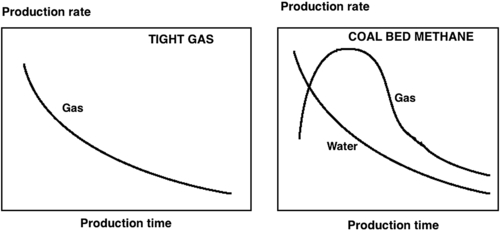
Figure 7.19 Conventional simulation techniques cannot simulate even fundamental features of various unconventional gas flow.
7.4. Comprehensive Modeling
This section introduces the governing PDEs that describe fluid flow in reservoir, where the matrix/fracture scheme controls the flow behavior. To represent flow behavior in porous media, suitable boundary and initial conditions must be considered and selected, and appropriate equations derived. Such governing equations describing the flow mechanism are the cornerstones of numerical modeling of an unconventional reservoir.
7.4.1. Governing Equations
In this section, the diffusivity equation of Forchheimer, the modified Brinkman Model, and the comprehensive model are discussed. Although modeled previously, Darcy's diffusivity equation is included because of its wide use throughout the oil industry. Here it will be used as a reference to compare its predictions with alternative models proposed herein. Forchheimer's model, popular in gas reservoirs' description, is used to derive a new diffusivity equation. What may be called modified Brinkman's model (MBM)—MBM's diffusivity equation incorporating both viscous and viscous/frictional terms from the original equation plus the inertial term from Forchheimer's basic equation—is also developed. The viscous terms of Brinkman's original equation are in fact Darcy's viscous term and another viscous/frictional term representing the forces generated by friction between layers of the fluid and its medium. The comprehensive is the ultimate proposed model; it has been called “comprehensive” because it includes all terms that might influence fluid flow in porous media in both Darcian and non-Darcian domains. It includes Darcy's viscous term, Forchheimer's inertial term, Brinkman's viscous/frictional term, and a Navier–Stokes convective term.
Although the situation of hydraulic fracturing, with the assumption of single horizontal fracture acting in the middle of a matrix system, can be modeled as a separate case, it is more appropriate to describe such a case using the models proposed in this section. Such models are valid for any hydraulic fracture aperture and length, any matrix size and extent; and also taking into account that inconsistent and heterogeneous matrix systems are highly preferable. Another unique model presented here deals with the coupled fluid flow/stress, and it should substantially enhance predictions of depletion while a reservoir is still in production. This model couples fluid flow conceptualization from this study with another stress model that updates petrophysical properties (porosity and permeability) according to effective stress variations arising from depletion, or other injection/flooding recovery techniques. Because, the model uses different flow equations in different sections of the reservoir, there is no need to make further assumptions.
7.4.1.1. Darcy's Model
Darcy's original equation (Eqn (7.6)) has been used to derive a diffusivity equation. This is the most commonly used equation in petroleum engineering analysis of well tests. This equation has also been used to predict reservoir pressure at any point of space and time within the reservoir. For single-phase linear flow, the pressure gradient in the x-coordinate is predicted by this equation:
∂2P∂x2=ϕμck∂P∂t
![]() (7.6)
(7.6)
where c, the total compressibility, is the sum of cf (fluid compressibility) and cr (rock compressibility).
In two dimensions, the diffusivity equation becomes:
∂2P∂x2+∂2P∂y2=ϕμck∂P∂t
![]() (7.7)
(7.7)
If the single phase considered flowing in the porous media is liquid, porosity (ϕ), permeability (k), viscosity (μ), and compressibility (c) are assumed to be constant. This assumption rests on the general and credible belief that liquids flowing in porous media are slightly compressible and the change in rock compressibility is negligible. Therefore, slight changes in these properties result in only negligible changes during flow. However, as will be seen in later section, this is not always the case. Many experimental investigations and field evidence show significant changes in rock properties during processes of depletion.
7.4.2. Forchheimer's Model
To develop a diffusivity equation similar to that of Darcy (Eqns (7.6) and (7.7)) for flow behavior replacing Darcy's linear equation by Forchheimer's nonlinear equation, consider an element of the reservoir through which a single phase (water, for example) is flowing in the x-direction and apply the conservation of mass balance equation (Figure 7.20):
Mass rate in − Mass rate out = Mass rate of accumulation.
In symbols:
(vxρxΔyΔz)−(vx+Δxρx+ΔxΔyΔz)=(ΔxΔyΔz)ϕ(ρt+Δt−ρt)Δt
![]() (7.8)
(7.8)
Dividing Eqn (7.8) by ΔxΔyΔz gives:
−(vx+Δxρx+Δx)−(vxρx)Δx=ϕ(ρt+Δt−ρt)Δt
![]() (7.9)
(7.9)
Take the limit as Δx and Δt go to zero simultaneously:
∂(vρ)∂(x)=−ϕ∂ρ∂t
![]() (7.10)
(7.10)
This is the continuity equation in a linear system. We may therefore write this equation in the y and z coordinates:
∂(vρ)∂(y)=−ϕ∂ρ∂t
![]() (7.11)
(7.11)
∂(vρ)∂(z)=−ϕ∂ρ∂t
![]() (7.12)
(7.12)
Taking the derivative of the left-hand side of Eqn (7.10) in two dimensions, we obtain:
ρ∂v∂x+v∂ρ∂x+ρ∂v∂y+v∂ρ∂y=−ϕ∂ρ∂t
![]() (7.13)
(7.13)
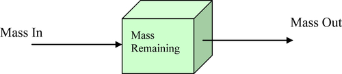
Figure 7.20 Schematic of the porous system considered for derivation of the diffusivity equation.
Now, Forchheimer's equation in the x-direction states:
−∂P∂x=μkv+βρv2
![]() (7.14)
(7.14)
and in the y-direction:
−∂P∂y=μkv+βρv2
![]() (7.15)
(7.15)
β is called the non-Darcy flow coefficient, Forchheimer's coefficient or turbulence coefficient, (1/ft). It is attributed to non-Darcy flow behavior. Several formulae are available for evaluating β, for example:
β=5.5×10⁹k5/4ϕ3/4
![]() (7.16)
(7.16)
Taking the derivative with respect to x of both sides of Eqn (7.14) and with respect to y of both sides of Eqn (7.15):
−∂2P∂x2=μk∂v∂x+2βρv∂v∂x
![]() (7.17)
(7.17)
−∂2P∂y2=μk∂v∂y+2βρv∂v∂y
![]() (7.18)
(7.18)
−∂2P∂x2=ρ(μkρ+2βv)∂v∂x
 (7.19)
−∂2P∂y2=ρ(μkρ+2βv)∂v∂y
 (7.20)
From Eqn (7.13):
ρ(∂v∂x)=−ϕ∂ρ∂t−v∂ρ∂x
![]() (7.21)
(7.21)
−∂2P∂x2=(μkρ+2βv)(−ϕ∂ρ∂t−v∂ρ∂x)
 (7.22)
Dividing both sides of Eqn (7.22) by (−1):
∂2P∂x2=(μkρ+2βv)(ϕ∂ρ∂t+v∂ρ∂x)
 (7.23)
∂2P∂x2=(μkρ+2βv)(ϕ∂ρ∂P∂P∂t+v∂ρ∂P∂P∂x)
 (7.24)
Rearrange Eqn (7.24):
∂2P∂x2=(μkρ+2βv)(ϕ∂P∂t+v∂P∂x)∂ρ∂P
 (7.25)
∂2P∂x2=(μkρ+2βv)(ϕ∂P∂t+v∂P∂x)cρ
 (7.26)
By rearrangement of Eqn (7.26):
∂2P∂x2=cϕ(μk+2ρβv)∂P∂t+cv(μk+2ρβv)∂P∂x
![]() (7.27)
(7.27)
Equation (7.27) is the nonlinear diffusivity equation in one dimension for the Darcy/non-Darcy (Forchheimer Model). It can be expressed in two dimensions:
∂2P∂x2+∂2P∂y2=c(μk+2βρv)(ϕ∂P∂t+v[∂P∂x+∂P∂y])
 (7.28)
7.4.3. Modified Brinkman's Model
The common belief is that non-Darcian behavior can be caused by a number of factors and not the inertial term suggested by Forchheimer alone. Three aspects of non-Darcian behavior have been addressed in this section. The model presented herein is based on the two terms included in the previously derived Forchheimer's model (Darcy's viscous and Forchheimer's inertial) and the viscous/frictional term introduced in Brinkman's basic equation.
Having derived a diffusivity equation based on Forchheimer's fundamental equation, a diffusivity equation based on a combination of Darcy's, Forchheimer's, and Brinkman's terms may be derived as following:
Consider the flow in the x-direction for now. The pressure drop in the x-direction would be affected by Darcy's, Forchheimer's, and Brinkman's terms. The fundamental equation inferred from this setup takes the following form:
∂P∂X=−μVK−ρβV2+μ′∂2V∂X2
![]() (7.29)
(7.29)
Rearrange:
∂2V∂X2=1μ′(∂P∂X+μKV+ρβV2)
 (7.30)
From the same Eqn (7.10), we can obtain:
ρ∂V∂X+V∂ρ∂X=−ϕ∂ρ∂t
![]() (7.31)
(7.31)
Take the derivative of both sides of Eqn (7.31) with respect to X:
ρ∂2V∂X2+∂V∂X∂ρ∂X+V∂2ρ∂X2+∂ρ∂X∂V∂X=−ϕ∂2ρ∂t∂X
![]() (7.32)
(7.32)
ρμ′(∂P∂X+μKV+ρβV2)+∂V∂X∂ρ∂X+V∂2ρ∂X2+∂V∂X∂ρ∂X=−ϕ∂2ρ∂t∂X
 (7.33)
Rearrange:
ρμ′∂P∂X+ρμμ′KV+ρ2βμ′V2+2∂V∂X∂ρ∂X+V∂2ρ∂X2=−ϕ∂2ρ∂t∂X
![]() (7.34)
(7.34)
Using chain rule for: ∂2ρ∂X2 we obtain:
∂2ρ∂X2=∂∂X(∂ρ∂X)=∂∂X(∂ρ∂P∂P∂X)=∂∂X(ρC∂P∂X)=ρC∂2P∂X2
 (7.35)
Same way we have: for: ∂2ρ∂t∂X we obtain:
∂2ρ∂t∂X=∂∂t(∂ρ∂X)=∂∂t(∂ρ∂P∂P∂X)=∂∂t(ρC∂P∂X)=ρC∂2P∂t∂X
 (7.36)
and for: ∂ρ∂X we obtain:
∂ρ∂X=∂ρ∂P∂P∂X=ρC∂P∂X
![]() (7.37)
(7.37)
C=1ρ∂ρ∂P
![]() (7.38)
(7.38)
Substitute for∂2ρ∂X2, ∂2ρ∂t∂X and ∂ρ∂X from Eqns (7.35), (7.36), and (7.37) respectively into Eqn (7.34):
ρμ′∂P∂X+ρμμ′KV+ρ2βμ′V2+2ρC∂V∂X∂P∂X+VρC∂2P∂X2=−ϕρC∂2P∂t∂X
![]() (7.39)
(7.39)
Effective viscosity “μ′” is defined as:
ρϕμ∂P∂X+ρϕKV+ρ2βϕμV2+2ρC∂V∂X∂P∂X+VρC∂2P∂X2=−ϕρC∂2P∂t∂X
 (7.40)
Divide both sides of Eqn (7.40) by ϕρC:
−1Cμ∂P∂X−1CKV−ρβCμV2−2ϕ∂V∂X∂P∂X−Vϕ∂2P∂X2=∂2P∂t∂X
![]() (7.41)
(7.41)
Again, using chain rule for ∂V∂X we obtain:
∂V∂X=∂V∂P∂P∂X
![]() (7.42)
(7.42)
Substitute in Eqn (7.41):
−1Cμ∂P∂X−1CKV−ρβCμV2−2ϕ∂V∂P(∂P∂X)2−Vϕ∂2P∂X2=∂2P∂t∂X
 (7.43)
∂P∂X is a small quantity and (∂P∂X)2
 is even smaller, therefore: (∂P∂X)2≈0
 , substitute in Eqn (7.43):
−1Cμ∂P∂X−1CKV−ρβCμV2−Vϕ∂2P∂X2=∂2P∂t∂X
![]() (7.44)
(7.44)
Equation (7.44) is the diffusivity equation in the x-direction, for the y-direction we obtain:
−1Cμ∂P∂Y−1CKV−ρβCμV2−Vϕ∂2P∂Y2=∂2P∂t∂Y
![]() (7.45)
(7.45)
−1Cμ(∂P∂X+∂P∂Y)−2CKV−2ρβCμV2−Vϕ(∂2P∂X2+∂2P∂Y2)=∂∂t(∂P∂X+∂P∂Y)
 (7.46)
7.4.4. The Comprehensive Model
In this section, the principle idea underlying the comprehensive model is introduced. This is translated into a mathematical form that can be easily used to describe fluid flow in porous media.
The idea is very simple: the Navier–Stokes equations, representing fluid flow between two parallel plates, are applied. Figure 7.21 schematically describes such a system.
Fluid flow between two parallel plates or in a pipe as described by the Navier–Stokes equations is well documented. The representative equations give highly accurate results. They have been used in many applications and modified to suit many other circumstances. The pressure gradient in the x-direction, as described by the basic Navier–Stokes equations, takes this form:
−∂P∂x=ρ(∂U∂t+U∂U∂x+V∂U∂y)
![]() (7.47)
(7.47)
In the y-direction, the pressure gradient takes the following form:
−∂P∂y=ρ(∂V∂t+U∂V∂x+V∂V∂y)
![]() (7.48)
(7.48)
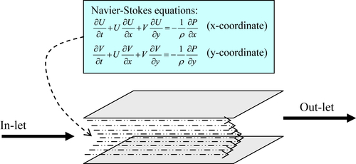
Figure 7.21 Schematic of fluid flow between two parallel plates described by the Navier–Stokes equations.
The summation of Eqns (7.47) and (7.48) is the total pressure gradient in two dimensions as described by the Navier–Stokes equations:
−(∂P∂x+∂P∂y)=ρ(∂U∂t+∂V∂t+U∂U∂x+V∂U∂y+U∂V∂x+V∂V∂y)
![]() (7.49)
(7.49)
Introducing grain particles in the space between the two plates (Figure 7.22) would hinder the flow and cause extra resistance forces against Navier–Stokes prescribed fluid flow. Hence, a modification is required to account for this resistance.
The full boundary layer equations were analyzed to investigate forced convection from a horizontal flat porous medium filling the space between the two plates described in Figure 7.23. The porous material is assumed to be 100% saturated with the flowing fluid. The Navier–Stokes equations are adapted from the case described in Figure 7.23, where the space between the two plates is occupied by both the volume of grains and the space left between the grain particles through which the flowing fluid runs. Obviously, the fluid will be flowing only through that space (pore space) between grain particles opposed by convective forces in addition to the other viscous, frictional, and inertial forces usually associated with fluid flow in a porous system. Therefore, the term “porosity” denoted by “ϕ,” become helpful in expressing the ratio of total pore space volume (space between grain particles) to the total volume of the system (total volume bounded by the two plates consists of both grain particles and pores in between):
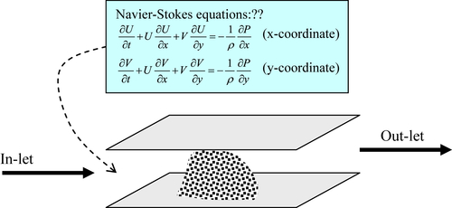
Figure 7.22 Schematic of fluid flow between two parallel plates with pile of grain particles in between causing extra resistance to flow.
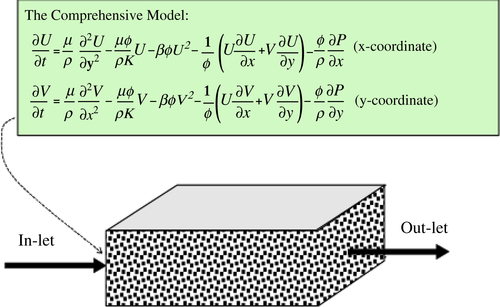
Figure 7.23 Schematic of fluid flow between two parallel plates filled with grain particles in between representing porous media flow.
ϕ=(PoreSpaceVolume)(TotalVolume)
![]() (7.50)
(7.50)
In fact, the pressure gradient mentioned in both Eqns (7.47) and (7.48) describes the situation where flow is subjected to the “total volume” between the plates. In the case considered in Figure 7.23, the convective forces are causing resistance to flow and contributing to a pressure gradient only within “pore space” through which the flow is actually taking place. We can define the pore space volume according to Eqn (7.50) then:
PoreSpaceVolume=ϕ×TotalVolume
![]() (7.51)
(7.51)
Hence, to express the effect of convective forces on the pressure gradient in the scheme represented by Figure 7.23, we should multiply by “ϕ” to determine how much of the bulk volume between the plates is exposed to the flow. So Eqns (7.47) and (7.48) become:
−ϕ(∂P∂x+ρ∂U∂t)=ρ(U∂U∂x+V∂U∂y)
![]() (7.52)
(7.52)
−ϕ(∂P∂y+ρ∂V∂t)=ρ(U∂V∂x+V∂V∂y)
![]() (7.53)
(7.53)
However, the pressure gradient is affected not only by the convection term from Navier–Stokes, but also by viscous forces (Darcy's term), inertial forces (Forchheimer's term), and the viscous frictional drag forces (Brinkman's term). Considering the contribution of these terms, the above equations would take the following form, in which the x-direction component becomes:
−∂P∂x=ρ(∂U∂t+1ϕ[U∂U∂x+V∂U∂y]+μKU+ρβU2−μϕ∂2U∂y2)
 (7.54)
The y-direction component becomes:
−∂P∂y=ρ(∂V∂t+1ϕ[U∂V∂x+V∂V∂y]+μKV+ρβV2−μϕ∂2V∂x2)
 (7.55)
∂U∂t=μρ∂2U∂y2−μϕρKU−βϕU2−1ϕ(U∂U∂x+V∂U∂y)−ϕρ∂P∂x
 (7.56)
∂V∂t=μρ∂2V∂y2−μϕρKV−βϕV2−1ϕ(U∂V∂x+V∂V∂y)−ϕρ∂P∂y
 (7.57)
7.5. Towards Solving Nonlinear Equations
Petroleum reservoir engineering problems are known to be inherently nonlinear. Consequently, solutions to the complete multiphase flow equations have been principally attempted with numerical methods. However, simplified forms of the problem have been solved some 60 years ago, when the Buckley–Leverett formulation was introduced. Ever since the pioneer work that neglected the capillary term, this formulation has been widely accepted in the petroleum industry. By using the method of characteristic, the multiphase one-dimensional fluid flow was solved. However, the resulting solution was a triple-valued one for a significant region. For decades, the existence of multiple solutions was considered to be the result of nonlinearity. Buckley and Leverett introduced shock utilizing the concept of material balance and two decades later, when numerical solutions were possible, it was discovered that the triple-value problem disappeared if the complete flow equation, including the capillary pressure form, is solved. Numerical methods, however, are not free from linearization. In fact, every numerical solution imposes linearization at some point of the solution scheme. Therefore, a numerical technique cannot be used to definitively state the origin of multiple solutions. In this section, a semianalytical technique, the Adomian decomposition method (ADM), capable of solving nonlinear PDEs without any linearizing assumptions, is used to unravel the true nature of the one-dimensional, two-phase flow. Results show that the Buckley–Leverett shock is neither necessary nor accurate portrayal of the displacement process. By using the ADM, the solution profile observed through numerous experimental studies was rediscovered. This paper opens up an opportunity to seek approximate but close to exact solutions to the multiphase flow problems in porous media.
7.5.1. Adomian Domain Decomposition Method
Since Adomian (1984) proposed his decomposition technique, the ADM has gained significant interests among researchers, particularly in the fields of physics and mathematics. They applied this method to many deterministic and stochastic problems (Adomian, 1986, 1994; Eugene, 1993). In this method, the governing equation is transformed into a recursive relationship and the solution appears in the form of a power series. The ADM has emerged as an alternative method to solve various mathematical models including algebraic, differential, integral, integro-differential, PDEs and systems, higher order ordinary differential equations, and others.
Guellal and Cherruault (1995) utilized the method to solve an elliptical boundary value problem with an auxiliary condition. Laffez and Abbaoui (1996) used it in modeling thermal exchanges associated to drilling wells. The application of this method is also noticeable in medical research, in which the decomposition technique is used to solve differential system of equations in modeling of HIV immune dynamics (Adjedj, 1999). Wazwaz (2001) and Wazwaz and El-Sayed (2001) reported that the ADM could be useful in solving problems without considering linearization, perturbation, or unjustified assumptions that may alter the nature of the problem under investigation. Also there have been suggestions that this method can be more advantageous over numerical methods by providing analytic, verifiable, rapidly convergent approximations that add insight into the character and the behavior of the solution as obtainable in the closed form solution (El-Sayed and Abdel-Aziz, 2003). In particular, they noticed the strength of the ADM in handling nonlinear problems in terms of rapid convergence. Biazar and Ebrahimi (2005) also expressed similar notion about rapid convergence and further added the advantage of the technique in terms of considerable savings in computation time when they attempted to solve hyperbolic equations.
Even though, petroleum problems are some of the most intrigue candidates for the ADM, there have been sparse attempts to utilize the method in the petroleum problems. Only recently, Mustafiz et al. (2005) reported the decomposition of the non-Darcy flow equations in porous media. In a different paper, Mustafiz and Islam (2005) transformed the diffusivity equations in well test applications into canonical forms. There is some success with ADM in modeling drilling activities, such as perforation by drilling (Rahman et al., in press) in specified drilling operations (Biazar and Islam, in press).
The Buckley–Leverett (1942) analysis is considered to be the first pioneer work in the study of linear displacement of a fluid by another fluid. The solution of their displacement study on two-phase fluid excluded the effect of capillary and gave multiple results for saturation at a given position. Realizing the fact that such coexistence of multiple saturation values is physically unrealistic, Buckley and Leverett (1942) used the fundamental concept of material balance to explain the shock. However, the lack of theoretical justification of shock was a major constraint in understanding the displacement phenomenon more vividly than before, and could not be reevaluated until the next significant work published by Holmgren and Morse (1951). They utilized the Buckley–Leverett theory to calculate the average water saturation at breakthrough and explained dispersion as a consequence of capillary effects. Welge (1952) continued the effort in finding the average saturation at water breakthrough in an oil reservoir. He also found that the method of tangent construction by Terwilliger et al. (1951) was equivalent to the shock proposed by Buckley and Leverett.
To solve the displacement equation including capillary as well as gravity, Fayers and Sheldon (1959) attempted a Lagrangian approach. They, however, did not succeed to determine the time required to obtain a particular saturation, which later was explained by Bentsen (1978) revealing the fact that the distance traveled by zero saturation is governed by a separate equation. Bentsen also noted that at slower injection rates, the input boundary condition of constant normalized saturation that Fayers and Sheldon used was incorrect in formulation. Also, there have been numerical investigations in the past to solve the displacement equation. Hovanessian and Fayers (1961) were able to avoid profiles of multiple valued saturations by considering the capillary pressure.
The ADM is applied to solve the nonlinear Buckley–Leverett equation. The solution for the water saturation is expressed in a series form. The base element of the series solution is obtained using the solution of the linear part of the Buckley–Leverett equation without the effect of the capillary pressure using the characteristic method. The other elements of the series solution are obtained recursively using the Adomian polynomial. The modification of the ADM in selection of the base element of the series solution makes the ADM feasible in solution of the nonlinear Buckley–Leverett equation. The computation is carried out for a reservoir of certain properties and initial conditions.
7.5.1.1. Governing Equations
The Buckley–Leverett equation is given by
∂Sw∂t+qAϕ∂fw∂Sw∂Sw∂x=0
![]() (7.58)
(7.58)
where fw is expressed in the form
fw=(11+kroμwkrwμo){1+Akkroqμo[∂Pc∂x−(ρw−ρo)gsinα]}.
 (7.59)
This equation indicates that the fractional flow rate of water depends on reservoir characteristics, water injection rate, viscosity, and direction of flow. The effect of capillary pressure, Pc, which appears in the fractional flow equation, on saturation profiles is important, since these profiles affect the ultimate economic oil recovery (Bentsen, 1978). The ratio of effective permeability to viscosity is defined as the mobility that is shown for water and oil, respectively.
λw=kkrwμwandλo=kkroμo.
![]() (7.60)
(7.60)
The mobility ratio of oil to water is defined by
M=λoλw=kroμwkrwμo.
![]() (7.61)
(7.61)
The assumptions associated with the Buckley–Leverett equation, according to Ertekin et al. (2001) are:
• oil and water phases are assumed incompressible;
• the porous medium is assumed incompressible, which implies that porosity is constant;
• injection and production are taken care of by means of boundary conditions, which indicate that there are no external sink or source in the porous medium;
• the cross-sectional area that is open to flow is constant;
• the saturation-constraint equation for two-phase flow is valid; and
• the fractional flow of water is dependent on water saturation only.
The expression of the fractional flow rate of water in Eqn (7.59) suggests that Eqn (7.60) is a nonlinear differential equation and it is due to the effect of capillary pressure. In the simplest case of horizontal flow and neglecting the effects of capillary pressure variation along the reservoir, the expression for fw in Eqn (7.59) is simplified to a linear differential equation, which is given by
fw=11+M.
![]() (7.62)
(7.62)
The water saturation distribution along the reservoir can be found at different time steps by knowing the injection flow rate, the initial water saturation distribution, and the variation of fractional water flow rate. The water is normally the wetting fluid in the water–oil two-phase flow systems. The relative permeability of the water and oil for a specific reservoir are obtained with the drainage and imbibitions process on the core in the laboratory. However, in this paper, the variation of relative permeability to water and oil as a function of water saturation are obtained using following empirical relationships respectively.
krw=α1Sn1wn
![]() (7.63)
(7.63)
kro=α2(1−Swn)n2
![]() (7.64)
(7.64)
Swn=Sw−Swi1−Swi−Sor
![]() (7.65)
(7.65)
If the effects of capillary pressure are included in a horizontal reservoir, Eqn (7.59) takes the form.
fw=11+kroμwkrwμo[1+Akkroqμo∂Pc∂x].
 (7.66)
Capillary pressure at any point is directly related to the mean curvature of the interface, which, in turn, is a function of saturation (Leverett, 1942). Therefore, it can be safely assumed that capillary pressure is only a function of water saturation. By applying the chain rule,
Pc=f(Sw)→∂Pc∂x=∂Pc∂Sw∂Sw∂x
![]() (7.67)
(7.67)
∂Sw∂t+qAϕ∂∂Sw(11+kroμwkrwμo)∂Sw∂x+kkroμoϕ∂∂Sw(11+kroμwkrwμo)∂Pc∂Sw(∂Sw∂x)2+kμoϕ(11+kroμwkrwμo)∂kro∂Sw∂Pc∂Sw(∂Sw∂x)2+kkroμoϕ(11+kroμwkrwμo)∂2Pc∂S2w(∂Sw∂x)2=0.
 (7.68)
Equation (7.68) is a nonlinear PDE and the nonlinearity arises because of the inclusion of capillary pressure in it.
7.5.1.2. Adomian Decomposition of Buckley–Leverett equation
In the ADM, the solution of a given problem is considered as a series solution. Therefore, the water saturation is expressed as
Sw(x,t)=∑∞n=0Swn.
 (7.69)
If a functional equation is taken into account for water saturation, it can be written in the form
∑∞n=0Swn=f(x,t)+∑∞n=0An.
 (7.70)
where f(x,t) is a given function and An (Swo, Sw1, Sw2,…., Swn) or, simply, Ans are called Adomian polynomials. The Adomian polynomials are expressed as
An=1n!dndλn[N(∑∞i=0λiSwn(x,t)i)]λ=0
 (7.71)
where N is an operator and λ is a parameter. The elements of the series solution for Swn(x, t) are obtained recursively by
Sw0(x,t)=f(x,t),Sw1(x,t)=A0,⋯Swk(x,t)=Ak−1⋯.
![]() (7.72)
(7.72)
By this arrangement, the linear and nonlinear part of the functional Eqn (7.70) is replaced by a known function using the recursive Eqn (7.72). By integrating Eqn (7.68) with respect to t
Sw=Sw(x,0)−∫t0[qAϕ∂∂Sw((11+kroμwkrwμo)∂Sw∂x)]dt−∫t0[kkroμoϕ∂∂Sw(11+kroμwkrwμo)∂Pc∂Sw(∂Sw∂x)2+kμoϕ(11+kroμwkrwμo)∂kro∂Sw∂Pc∂Sw(∂Sw∂x)2+kkroμoϕ(11+kroμwkrwμo)∂2Pc∂S2w(∂Sw∂x)2]dt.
 (7.73)
Comparing Eqn (7.73) with Eqn (7.70) and taking into account of Eqn (7.72), the elements of the water saturation series are obtained.
Sw0(x,t)=Sw(0,x)−∫t0[qAϕ∂∂Sw0(11+kroμwkrwμo)∂Sw0∂x]dtSw1(x,t)=−∫t0[kkroμoϕ∂∂Sw0(11+kroμwkrwμo)∂Pc∂Sw0+kμoϕ(11+kroμwkrwμo)∂kro∂Sw0∂Pc∂Sw0+kkroμoϕ(11+kroμwkrwμo)∂2Pc∂S2w0](∂Sw0∂x)2dtSw2(x,t)=−ddλ∫t0[kkroμoϕ∂∂(Sw0+Sw1)(11+kroμwkrwμo)∂Pc∂(Sw0+Sw1)+kμoϕ(11+kroμwkrwμo)∂kro∂(Sw0+Sw1)∂Pc∂(Sw0+Sw1)+kkroμoϕ(11+kroμwkrwμo)∂2Pc∂(Sw0+Sw1)2](∂(Sw0+λSw1)∂x)2dtSw3(x,t)=12!d2dλ2∫t0[kkroμoϕ∂∂(Sw0+Sw1+Sw2)(11+kroμwkrwμo)∂Pc∂(Sw0+Sw1+Sw2)+kμoϕ(11+kroμwkrwμo)∂kro∂(Sw0+Sw1+Sw2)2∂Pc∂(Sw0+Sw1+Sw2)+kkroμoϕ(11+kroμwkrwμo)∂2Pc∂(Sw0+Sw1+Sw2)2](∂(Sw0+λSw1+λ2Sw2)∂x)2dt⋯⋯⋯⋯⋯⋯⋯⋯
 (7.74)
7.5.3. Discussion
The method is applied to a given reservoir with the initial water saturation of 0.18. This value is corresponding to the irreducible water saturation of the reservoir. Water is injected into the reservoir with a linear flow rate of 1 ft/day. The oil and water viscosities are 1.73 and 0.52 cp, respectively. The flow of the displaced phase (oil) ceases at Soc = 0.1. The porosity of the medium is 0.25 with an absolute permeability of k = 10mD.
The normalized water saturation and the water and oil relative permeability are obtained using
Swn=Sw−0.181−0.1−0.18,krw=0.59439S4wn,kro=(1−Swn)2
![]() (7.75)
(7.75)
A typical plot of variation of relative permeability to water, krw, relative permeability to oil, kro, fractional flow curve, fw and its derivative, dfw/dSw are shown in Figure 7.24. The capillary pressure data are also shown in Table 7.1.
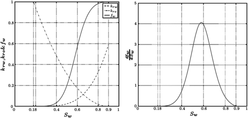
Figure 7.24 The variation of the water and oil relative permeability, the fractional water flow rate, and the differentiation of fractional water flow rate with the water saturation.
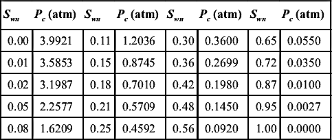
The solution for the first base element of the series solution of the water saturation,Sw0, is obtained through the solution of the first equation in Eqn (7.74). It can be written by integrating from the both sides of the first equation in Eqn (7.74) and using Eqn (7.61) that
∂Sw0∂t+qAϕ∂∂Sw0(11+M)∂Sw0∂x=0.
![]() (7.76)
(7.76)
This equation suggests that Sw0 is constant along a direction that is called characteristic direction. The characteristic direction can be obtained by
(dxdt)Sw0=qAϕ∂∂Sw0(11+M)t.
 (7.77)
that is the Buckley–Leverett frontal advance equation. Integrating with respect to time, the distribution of Sw0 is found in the form of
x(t,Sw0)=qtAϕ∂∂Sw0(11+M)t.
![]() (7.78)
(7.78)
The solution of Eqn (7.68) gives the variation of the Sw0 along the reservoir at certain time. The distribution of Sw0 along the reservoir is obtained based on the definition of the mobility ratio Eqn (7.61) and the relations for the relative permeability of water and oil in Eqn (7.75). It corresponds to the variation of the water saturation when the effect of the capillary pressure is ignored. The computations are carried out at different time of t = 0.5, 1, 2, 5,and 10 days. The solution for the water saturation without the capillary pressure effect shows the unrealistic physical situation that Buckley–Leverett mentioned in their pioneer paper with multiple saturations at each distance (x-position) as given partly in Figure 7.25. In order to avoid multiple saturation values at a particular distance, a saturation discontinuity at a distance, xf, is generally created in such a way that the areas ahead of the front and below the curve are equal to each other.
The other elements of the series solution for the water are obtained recursively using Eqn (7.74) and the solution forSw0. The solution for Sw1 is obtained using the solution of Sw0 at a certain point for a given time. To induce the nonlinear dependence of capillary on saturation, during decomposition, the capillary pressure and its derivatives are approximated by using the cubic spline, as shown in Figure 7.26. The interpolating splines are preferred over interpolating polynomials as they do not suffer from oscillations between the knots and are smoother and more realistic than linear splines (Ertekin et al., 2001). Such technique is also used to observe the effects of linearization in pressure in reservoir flow equations (Mustafiz et al., 2006). The solutions for Sw2 and Sw3 are obtained recursively using Eqn (7.74). The computations show that the series solution converges very fast and it is not necessary to go further thanSw3.
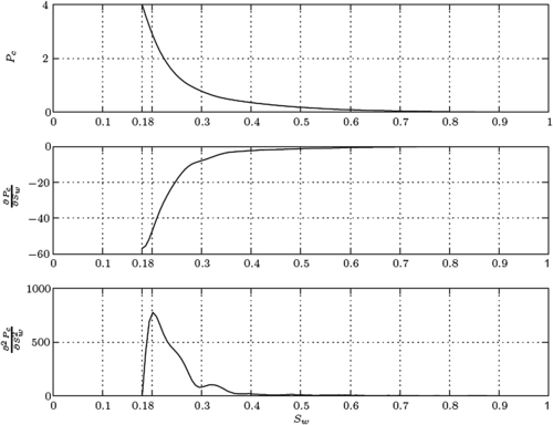
Figure 7.25 The water saturation distribution with and without the effect of capillary pressure using ADM.
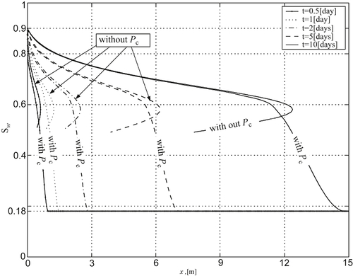
Figure 7.26 The capillary pressure variation and its first and second derivatives as a function of the water saturation.
The distribution of the water saturation along the reservoir is given in Figure 7.26. The results of the water saturation without the effect of the capillary pressure are also depicted in Figure 7.26 for the sake of comparison. This figure shows that by considering the effects of capillary pressure, it is possible to avoid unrealistic multiple saturation values. Moreover, the decomposition approach shows notable prediction of saturation profiles along the length. The gradual and mild changes observed in the saturation profile here, are perhaps less severe than the conventional prediction of shock-fronts.
..................Content has been hidden....................
You can't read the all page of ebook, please click here login for view all page.