10 High-Performance and Customizable Bioinformatic and Biomedical Very-Large-Scale-Integration Architectures

Very-large-scale-integrated circuits (VLSIs) and field-programmable gate arrays (FPGAs) are definitely competitive in computation-intensive applications, benefiting from their inherent parallelism, customizable property, and low power consumption. They are mostly employed to accelerate various algorithms since their introduction, by which large design space can be obtained to explore different levels of parallelization.

In this chapter, three key objectives are focused on: (1) The computing power and potential of parallel VLSI architectures in applications of bioinformatics and biomedical engineering are revealed and discussed. (2) According to intrinsic bottleneck of algorithms, parallel computing can be generalized into data-intensive and compute-intensive problems. Two successful bioinformatic and biomedical VLSI architectures are presented, which are representatively data-intensive and compute-intensive, respectively. The first one is a parameterizable VLSI architecture for geometric biclustering (GBC), which is a data mining technique allowing simultaneous clustering of the rows and columns of a matrix. The architecture is also scalable with the size of column data and the resources provided on FPGA. Compared with CPU implementation, it achieves considerable acceleration as well as low energy consumption. The second one is a hardware architecture for the stochastic state point process filter (SSPPF), which is an effective tool for coefficients tracking in neural spiking activity research. This architecture is scalable in terms of both matrix size and degree of parallelism. Experimental result shows its superior performance comparing to the software implementation, while maintaining the numerical precision. (3) Design techniques for different parallelism levels are classified and discussed. Hybrid design techniques are employed in the architectures to achieve multilevel parallelism exploration. This also provides a macroscopic view into high-performance architecture design.

10.1 Emerging Bioinformatics and Biomedical Engineering

10.1.1 Bioinformatics and Biomedical Algorithms

Nowadays, bioinformatics and biomedical engineering have become indispensable parts of modern life. The bioinformatics integrates biological information and newly updated computational technologies, and the target is to undertake two major tasks [1]. The first is to retrieve and organize data to allow researchers to readily access and manage existing information. In genetics and genomics research, for instance, the sequencing technique provides a way to determine the sequence of nucleotide bases in a DNA molecule. The famous comprehensive database GenBank contains nucleotide sequences that are publicly available for more than 260,000 named organisms [2]. The National Center for Biotechnology Information builds and maintains the GenBank with data obtained from worldwide individual laboratories, or from large-scale sequencing projects. The second task is to develop methodologies and tools to facilitate the analysis of biological data. This purpose is oftentimes achieved by applying well-developed algorithms or computational software/hardware, which could be in computer science or applied math, into the analysis process. One example is the Burrows–Wheeler transform [3], an algorithm employed in data compression, which has been successfully applied to DNA sequence alignment [4] such as the well-known tools Burrows–Wheeler Aligner [5] and Bowtie 2 [6].

Similarly, biomedical engineering is also a multidisciplinary field, utilizing engineering principles (such as electrical, chemical, optical, mechanical) to understand, modify, or control biological systems for the purpose of health care. Taking the neural coding problem for example, new techniques such as high-density multielectrode array recordings and multiphoton imaging techniques [7] make it possible to record from hundreds of neurons, rather than the previous repeated single neuron stimulating. Neurons can be characterized as electrical devices and can be directly analyzed as information processing devices using signal processing theory [8]. In addition, the neural coding is a fundamentally statistical problem since neural responses to stimuli are stochastic. Therefore, many classical statistical methods, which are widely utilized in communication and signal processing area, have been applied to build models to describe neural behavior [9].

Being extraordinary extensive fields, the major research of bioinformatics covers sequence analysis, gene expression analysis, computational evolutionary biology, and so on. On the other hand, biomedical engineers focus on a broader domain [10]. Some representative subdisciplines include biomechanics, prosthetic devices and artificial organs, neural engineering, and genetic engineering. In this chapter, we mainly focus on the specific problems of bio-sequence analysis and neural coding applications.

Analysis for bio-sequence such as DNA, RNA, and protein sequence is one of the most promising and challenging tasks [11]. Specifically, it refers to analyze the sequences to reveal the functions, structures, or mutations. This hidden gene information in the nucleotide sequence is in charge of encoding proteins for organs. Such analysis enables us to explore similarities between different species and to discover fatal diseases that oftentimes represent in forms of DNA base mutations. The technique has been widely applied into personalized medicine, biological research, and forensics. Some major types of these analyses consist of (1) DNA/RNA sequence alignment, which is meant to identify similarities between two or multiple sequences or to map short sequences to a reference genome database; (2) biclustering, originally for data mining application, which is an important method to analyze large-scale biological sequence set [12]; (3) sequence assembly, which is to construct the original DNA sequence with small fragments after sequencing process; and (4) phylogenetic analysis of DNA or protein sequences, which is an important method to find the evolutionary history of organisms from bacteria to humans [13].

The study of neural coding refers to searching and characterizing the correlations between neural action potentials or spikes and external-world sensory stimuli, motor actions, or mental states. The coding involves encoding and decoding corresponding to two opposite mapping directions [9]. The encoding is to predict the spike response of neurons to various types of stimuli. Conversely, the decoding problem concerns the estimation of the stimulus that gave rise to certain neuronal pattern. The neural coding algorithms need to characterize the models of neural spiking activity, which is a stochastic point process. Therefore, statistical theory, probability methods, and stochastic point processes are always applied in this field.

10.1.2 High-Performance Computing Requirements

In general, the major critical areas of requirement for the use of high-performance computing (HPC) in bioinformatics and biomedical research include (1) organizing, managing, mining, and analyzing the large volume of biological data; and (2) modeling and simulation, particularly in multiscale problems (modeling from the neuron, genome to the organism) [14]. The following sections will illustrate these requirements specifically.

Massively parallel next-generation sequencing techniques together with the need of gene expression analysis have resulted in a huge explosion in the amount of digital biological data. For around 20 years recently, the sizes of the genomic banks have experienced an exponential growth. Figure 10.1 is a picture of GenBank Statistics [15], which illustrates the growth of GenBank from its inception to 2013. The number of bases in GenBank has doubled approximately every 18 months. The size of the famous protein database—UniProtKB/TrEMBL—has increased by about 380 times from 1996 to 2013 (Release 1, November 1996). It retains 39,870,577 sequence entries consisting of 12,710,398,609 amino acids according to the latest release statistics (Release 2013_07) [16].

Furthermore, the improvement of sequencing machines and other progress in bio-technologies would further promote the future growth of biological databases. Thus, the essential problem is that the analysis of resulting data is unable to keep up with the producing pace. Thus, the processing of this avalanche of data to transform them into biological understanding is a significantly challenging task. Nowadays, most bioinformatics analysis tools are running on general purpose CPU platforms that are no longer scalable to the ever growing rate of publicly available data. Current approaches to this problem using conventional computers may take tens to hundreds of thousands of CPU hours to complete the alignment requirements for a single human genome. Hence, there is a need for faster computing platforms to cope with the database growth and people begin to resort to HPC to accelerate the processing and reduce bulk of computing time.

Except the requirement from biological data, in other applications, such as the neural modeling, the complexity of neural models continues to increase when realistic conditions and attributes, to emulate models for more accurate assessment of the actual model, are incorporated, such as larger populations, varied ionic conductances, more detailed morphologies, and so on [17,18]. Neural modelers often increase the computational requirements by orders of magnitude, which is often constrained by the limited performance of conventional personal computers. Therefore, HPC platforms and tools are desperately needed to facilitate such research.

Images

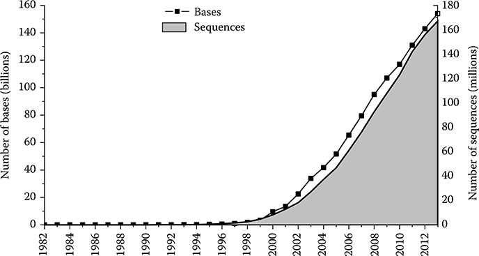
FIGURE 10.1 The graph depicts the number of bases and the number of sequence records in each release of GenBank, beginning with Release 3 in 1982. (Data from National Center for Biotechnology Information, accessed September 15, 2013, http://www.ncbi.nlm.nih.gov/genbank/statistics.)

HPC is defined as a set of hardware and software techniques developed to build computer systems capable of rapidly performing large amounts of computation. These techniques generally rely on harnessing the computing power of large numbers of processors working in parallel, either in tightly coupled shared-memory multiprocessors or loosely coupled clusters of PCs. Emerging HPC platforms such as FPGAs [4], Cell Broadband Engine [19], and graphics processing units [20] have been explored in biology-related research. In famous HPC centers such as San Diego Supercomputer Center [21] and Pittsburgh Supercomputing Center [22], bioscience applications occupy a large portion of computation missions.

10.2 High-Performance Very-Large-Scale Integration

10.2.1 Need for Very-Large-Scale Integration in High-Performance Computing

According to the so-called Moore’s Law, the performance of microprocessors has doubled every 18 months or so during the past four decades [23]. Although the conventional CPUs have experienced a significant improvement on computing performance, many limitations or bottlenecks still remain preventing them to successfully keep up with the demands from HPC applications. Simply increasing in clock rates and instruction-level parallelism could hardly be delivered further, because transistors are reaching the limits of miniaturization under current semiconductor technology. Besides, the memory bandwidth and disk access speeds could not match the ever-increasing CPU speeds completely, while the techniques to reduce the memory latency bottleneck are at the expense of extra circuitry complexity.

Currently, general-purpose CPU vendors change the strategy to rely on multicore and multithreaded architecture, to continue the proportional scaling of performance [24]. This design helps manage the thermal dissipation, because when frequency increases, power consumption escalates to impractical levels [25]. However, to take advantage of this parallelism, sophisticated hardware and developing software tools are required. Thus, the shift to multicore multithreaded paradigms introduces overhead and will not guarantee a linear enhancement in speed with increased number of processors because the memory bandwidth bottleneck has not been fully addressed.

To fill the enlarged gap between HPC requirement and limited CPU performance, heterogeneous systems are emerging, which are augmented hardware accelerators as coprocessors, as an alternative to CPU-only systems [25]. Very-large-scale-integration (VLSI) technology provides several custom solutions for application-oriented accelerators such as application-specific integrated circuit and FPGA. The conventional CPUs require decoding instructions and transferring data from cache or internal memory, which occupy a large portion of the overall computing process [26]. In contrast, application-specific VLSI could customize the pipeline, instruction flow, and data structure in correspondence with certain applications. Nevertheless, the hardware coprocessor faces a challenge that restraints its adaptability: the payback of designing a circuit for one application is low due to the long development time and high research and development costs [23].

The FPGA is an attractive solution to enlarge the diversity of applications. An FPGA consists of a large array of configurable logic blocks, block random-access memory (RAM), digital signal processing blocks, and input/output blocks [25]. The reconfigurability makes it suitable to a variety of applications. Containing a massive amount of programmable logic, FPGAs are able to provide different levels of parallelism: multiple processing elements (PEs) can be created in one single chip and work at the same time; dataflows between different operators can be controlled and streamed clock by clock; efficient pipeline architectures of variable depth are supported; on-chip memory reduces the bandwidth bottleneck for memory access. Besides, the FPGA is also a competitive candidate in embedded applications because of its power efficiency. All these properties have guaranteed the unshakable position of FPGAs in HPC community.

10.2.2 High-Performance Multilevel Parallel Designs

To outperform general-purpose CPUs, reconfigurable computers require techniques to design architectures that are efficient enough and achieve maximal parallelism. It means in each algorithmic step, the number of clock cycles is small while the computation carried out is as much as possible. The clock frequency is typically in the range of 2 to 3 GHz for high-performance processors. However, the hardware architectures always operate between 100 and 300 MHz for state-of-art FPGAs. Therefore, reconfigurable computers have to overcome a 10 times performance deficit to compete with CPUs.

There are several levels of parallelism to explore [27,28], which are enumerated as follows:

Task-level parallelism: Conventionally exploited by cluster computing, which is achieved by making each processor execute a respective thread on the same or different data set. It concerns the number of coarse-grained tasks that can be executed in parallel for FPGAs.
Instruction-level parallelism: Only a limited number of instructions can be executed on conventional processors. With much deeper pipelining controlled cycle by cycle, FPGAs can therefore support a variety of simultaneously executing in-flight instructions.
Bit-level parallelism: This parallelism is achieved by increasing processor word size. In hardware, customizable bandwidth of data and instruction can be set according to specific requirement.
Data-level parallelism: Divide and Conquer method, which refers to spreading the data onto different processing nodes that all carry out the same instructions. The FPGAs can take advantage of the fine-grained architecture for parallel execution. Multiple PEs could be constructed to execute on a large number of data sets simultaneously. Therefore, the equivalent performance of plenty of conventional CPUs can be achieved in a single FPGA chip.

By exploiting efficient mapping of all these levels of parallelism to the fabric, an FPGA operating at 200 MHz can outperform a 3 GHz processor by orders-of-magnitude or more, with greatly reduced power consumption [29]. Other definitions of types of parallelism such as kernel-level, problem-level, loop-level, expression-level parallelism, and so on [30,31] exist. They are specific to certain applications and can be covered by the four basic parallel types, thus are not elaborated here.

Other than parallelism level, parallelism is also classified in the term of granularity, which means the ratio of computation in relation to the amount of communication. Based on that, fine-grained, coarse-grained, and embarrassing parallelism is derived according to the order of decreasing in frequency of data communication among processors. The finer the granularity, the greater the potential for parallelism and hence speed-up would be achieved, but the higher the overheads of synchronization and communication.

The VLSI/FPGA parallel architectures are customizable and application specific. Different applications require specific computations and data structures, thus various unique parallel designs should be employed to meet these requirements. Therefore, to design a specific hardware architecture, the types of applications need to be summarized and classified. A technical report from UC Berkeley [32] had summarized 13 basic classes of problems that are explored by high-performance parallel architectures. They referred each class as a dwarf, which is a set of algorithms classified by similarity in computation and data movement, or memory access modes. Such classification is far different from other classification methods by subjects. From the perspective of parallel computing, however, this high-level abstraction allows reasoning about the dwarves’ behavior across a wide range of applications. Subjects, algorithms, together with hardware platforms evolve with time, but the underlying computation and data flow patterns remain still into the future.

Images

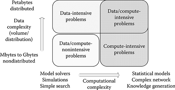
FIGURE 10.2 Classification of the application space between data-intensive and compute-intensive problems. (From Gorton, I. et al., Computer, 41(4), 30–32, 2008. With permission.)

From a macroscopic perspective, parallel computing applications can also be generally classified as data intensive and compute intensive [33]. Data-intensive application refers to processing and managing massive amounts of data volumes by parallel computing, and associated data analysis cycles are significantly reduced so that decisions can be made fast and timely [34]. Most of the execution time is spent on input/output (I/O) or memory transferring, so data-intensive applications are data-path oriented. The data volumes could be in size of terabytes or petabytes collected from experiments or simulations. Processing requirements usually scale near linearly according to data size and are normally amenable to straightforward parallelization methods. In contrast, compute-intensive computing devotes most of execution time to complex computation with smaller volumes of data required. Processing requirements normally scale superlinearly with data size [33]. Figure 10.2 shows a diagram to illustrate the application space between these problems [33]. Generally, there is always an overlap between these two types of computing.

In the following sections of this chapter, two high-performance parallel architectures in bioinformatics and biomedical engineering have been selected because they are representative in parallel computing: one is a data-intensive application and the other is a compute-intensive application. They also belong to two different dwarves in the Berkeley report [32]: the former comes from the Graph Traversal dwarf, and the second comes from the Dense Linear Algebra dwarf. Parallel techniques for each problem differ greatly. The techniques for data-intensive problem often involve decomposing or partitioning the big data into multiple segments and distributing to PEs. Each PE independently stores a segment and is responsible for computing its value. In this case, nonlocal communication should be minimized. This partition method is consistent with the definition of data-level parallelism. The more efficient the data be subdivided and distributed, the finer granularity can be explored in parallel processing. On the other side, compute-intensive processing usually involves task-level or bit-level parallelism. Because the data flow in compute-intensive problems is typically treated as a whole, parallelization should be performed within an application or an algorithm flow. The overall process can be resolved into separated distinct tasks and executed in parallel on appropriate platforms. If data dependency between successive steps exists and serial processing is unavoidable, bit-level or instruction-level parallelism would be exploited efficiently.

Indeed, more than one parallel technique is employed in each example. Exploiting parallelism at a single level is not an optimal solution and it would be wiser to use hybrid parallelism at all design levels. The hybrid design method is illustrated in detail in the following sections.

10.3 Scalable Very-Large-Scale-Integration Architecture for Data-Intensive Example

The data-intensive applications are becoming central to discovery-based science, especially in bioinformatics [35]. High-performance VLSI architectures are thus explored widely. In this section, a scalable GBC accelerator for DNA microarray data analysis is introduced. The bio-data analysis is a proper data-intensive application because the DNA database presents an exponential growth rate as aforementioned. The algorithm in GBC problem is not that complex. However, the large data volume involved makes the architecture design challenging. In this example, both data-level and task-level parallelism are explored efficiently.

10.3.1 Introduction to Geometric Biclustering

In the past decade, genomic data analysis has become one of the most important topics in biomedical research. Biologists correlate the gene information with diseases. For example, a cancer class can be discovered based on tissue classification [36]. Genes that have similar expression patterns may have common biological functions. There can be tens of thousands of genes involved in a microarray experiment, so efficient data analysis methods are indispensable for finding similar gene expression patterns. Figure 10.3 describes the flow of the gene analysis from expressing the genes to DNA microarray for pattern analysis.

Biclustering is an important method to analyze large biological and finical datasets [37,38], which is a process that partitions the data samples based on a number of similar criteria so that the existing patterns in the data can be analyzed. The biclustering process can be formulated in multidimensional data space for analysis [37].

Images

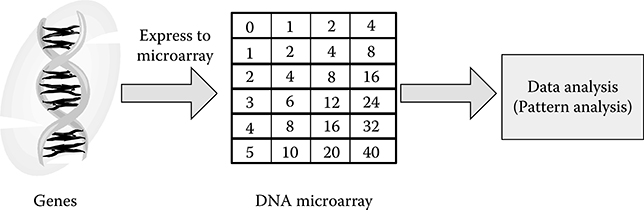
FIGURE 10.3 The flow of expressing a gene to a DNA microarray for data analysis.

GBC algorithm [39] identifies the linearities of microarray in a high-dimensional space of biclustering algorithm. It provides higher accuracy and reduces the computational complexity for coherent pattern detection compared to other methods. A hypergraph partitioning method [40] is proposed to further optimize the performance of the GBC algorithm. This method reduces the size of matrix in each operation to speed up the GBC algorithm using a software partition tool called hMetis. However, it is still time-consuming to search for the patterns of large-scale gene microarray data. A 100 by 100 matrix requires 2.8 minutes to identify the biclusters using the hypergraph partitioning method processed by the MATLAB program that runs on a machine with an Intel Core i7-920 2.66 GHz processor and DDR3 3 GB memory. But a normal gene matrix can have more than 10,000 rows or columns. Therefore, it is essential to accelerate this process [20].

10.3.2 Geometric Biclustering Algorithm

10.3.2.1 Geometric Biclustering Work Flow

Figure 10.4 shows the overall flow of the GBC algorithm. The microarray data is converted to two-dimensional column-pair space sub-biclusters by using the Hough transform (HT) and additive and multiplicative pattern plot (AMPP) [39]. The HT detects linear data points and forms sub-biclusters in column-pair space. AMPP classifies the collinear points in sub-biclusters for different patterns. The column-pair biclusters are combined to maximal biclusters, and the number of genes in the merged biclusters is reduced in this process. In the evaluation of the maximal biclusters, the biclusters are filtered out if the number of conditions is fewer than the given parameter. Finally, the valid maximal biclusters are the target search patterns.

Assume there is an m by n data matrix. In column-pair space, each column forms a column pair with all other columns. There are (n)(n – 1)/2 column pairs in total. Figure 10.5 illustrates an example of transforming a 5 by 4 data matrix (M_C) to a 5 by 6 column-pair matrix (M_S) in the GBC work flow. The target is finding an additive coherent pattern in the data matrix, where the value of the next column is equal to the value of the current column plus a constant (Ci = Cj + constant). The input matrix M_C is transformed to M_S by using HT and AMPP for additive coherent value. For example, column pair S_1,2 in M_S represents the comparison of C1 and C2 in M_C. The value “1” in S_1,2 indicates there is an additive coherent relationship of that position in C1 and C2. All the column pairs in M_S are combined in the combination process.

Images

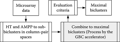
FIGURE 10.4 The work flow of the geometric biclustering algorithm.

Images

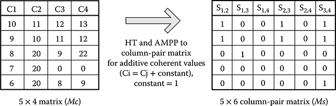
FIGURE 10.5 Example of transformation from data matrix to column-pair matrix. The set bit (logic ‘1’) in M_S represents two points at the two columns in M_C have coherent relationship.

10.3.2.2 Geometric Biclustering Combination Process

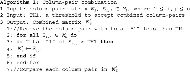
The combination algorithm is shown in Algorithm 1. Assuming that M_C is an m by n gene data matrix. The transformed column-pair matrix M_S contains R = (n) (n – 1)/2 column pairs in total. The column pairs are denoted as [S_1,2, S_1,3 … S_i,j], where 1 ≤ i,j ≤ n. The column is represented in a bit vector that only contains logic “0” or “1.” The threshold value TH1 is used to determine whether the combined column pair is valid or not. This threshold controls the sensitivity of the matching. Higher threshold value allows matching of less similar patterns. First, the column pairs that contain the number of “1” less than TH1 are eliminated to reduce the number of combines. Next, all the remaining column pairs are combined. The combined column pairs are included in M′_s if they are valid. The combination process is finished after all column pairs are visited. Figure 10.6 illustrates an example of the combination of the column-pair matrix in Figure 10.5. In each step of the process, two column pairs (S1, S2) are selected with common column in M_C to combine, and the column pair has at least one column different to other one. For example, S_1,2 and S_1,3 are common in column C1 in M_C and different in column C2 and column C3, then they can be combined. The visited S1 will not be selected again. S2 is combined with S1 by using arithmetic AND logic to S_combine. If the number of “1” in S_combine is greater than or equal to TH1, it is included in M_temp. After visiting all S2, M_temp is joined with M′_S. Then, the process selects next S1 for combination.

Images

After visiting all S1 in M′_S, evaluation criteria selects the maximal biclusters from M′_S. The elements in M′_S with a maximum number are chosen as the final solution. In the example of a column-pair matrix in Figure 10.5, S_1,2,3,4 is obtained as the maximal column pairs with column value [11000]. This represents the maximal bicluster containing columns [C1, C2, C3, C4] in the original matrix M_C, the position with value “1” is selected. The final additive coherent matrix after masking M_C with the bit matrix [39] can be obtained. This is the most computational intensive part of the GBC algorithm, which consumes over 80% of the computation time. Therefore, the aim is to accelerate this process.

Images

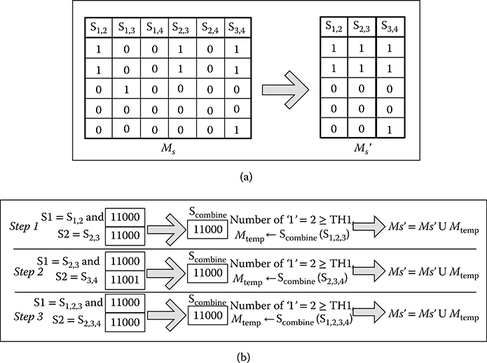
FIGURE 10.6 Example of combining a column-pair matrix, assuming TH1 = 2. (Ms). (a) Remove the column-pairs with total ‘1’ less than TH1 (Ms’), and (b) combine each column-pair in Ms’.

10.3.2.3 Parallelism Exploration for the Geometric Biclustering Combination Process

The combination process is the most time-consuming part in the GBC algorithm. It involves combining two column pairs each time. It is obvious that this process can be speeded up by combining several two column pairs at the same time. In the example in Figure 10.6, no data dependency is found for these two column pairs: S_1,2, S_1,3 and S_1,2, S_1,4, the selected input is independent to the output at the same processing cycle. Given this, the column pairs can be divided and processed by multiple PEs running side by side in parallel. Data-level parallelism is thus easily achieved. This parallelism can also be treated as task level because each column-pair combing process can be seen as an independent task. For example, Step 1 and Step 2 in Figure 10.6 can be processed in the same cycle. S_1,2,3 is dependent on S_1,2, S_1,3, and S_2,3, therefore the process of S_1,2,3 must be after combining all S_1,2, S_1,3, and S_2,3. The parallel ability of FPGA can facilitate this process.

Data-intensive problem often face the problem of I/O bandwidth [41] as the conventional CPUs. The gap between off-chip memory and processing units can significantly diminish the parallel advantage, due to the fact that huge data volume could not be stored cost-effectively on chip. Fortunately, the reconfigurability of FPGAs enables us to configure as many pins as possible to be I/O ports. In this design, only a 64-bit wide interface is dedicated to communicate with external memory because of reality restrictions.

10.3.3 Architecture Design

10.3.3.1 Architecture

A scalable GBC accelerator to facilitate the parallelism of the GBC algorithm is proposed. Figure 10.7 shows the architecture of GBC accelerator; the column pairs in matrix M_S are stored in external memories. There are four main components in the FPGA design to process the Algorithm 1; they include (1) Memory controller, (2) Clock management, (3) Data controller, and (4) N PEs.

The memory controller handles the read/write signals and sequence of data transferring to and from the external memory. It is the interface between external memory and data controller. The number of read port (Port_R) and write port (Port_W) depends on the external memory.

The clock management generates different clocks required for memories (memory clock), PEs (PE clock), and internal logics (system clock).

The data controller contains four units to process the combination process. First, S1, S2 selection unit selects the column pairs S1, S2 as in Algorithm 1. Second, PE management unit manages the available PEs to process the combination, distributes the selected column pairs to PEs, and collects the combined result S_combine. Third, data R/W unit asserts the read/write signals and handles the column pair’s data reading/writing for the memory controller. Fourth, state machine controls different states of the accelerator such as initialization and the finish of process.

The accelerator contains at most N PEs processing at the same time. The architecture of each PE is described in Figure 10.8, which consists of an independent set of FIFOs to store the two input column pairs (S1, S2) and the combined column pairs (S_combine). This distributed local memory makes the parallel process more efficient by keeping the balance of data transfer rate between external memory and PEs. The combine logic in the PE executes a bitwise AND operation for the two input column pairs. The count “1” logic is a shift register, a k-bit decoder (decode to log₂ k-bit) to check the number of “1” in AND_RESULT register, and an adder to sum up all the “1” values. Meanwhile, the AND_RESULT is stored in Result_FIFO for writing S_combine to memory. The threshold comparer checks if the combination is valid. The combination is valid if the total number of logic “1,” which is stored in register NUMBER_ONE, is greater than or equal to the threshold TH1. The state machine counts the total number of bytes combined by using a counter and asserts signal done when the combination of two column pairs is finished.

Images

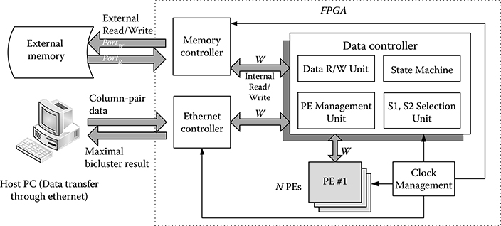
FIGURE 10.7 The architecture of geometric biclustering accelerator. W is the data width, N is the maximum number of processing elements, Port_R is the number of memory read port, Port_W is the number of memory write port.

Images

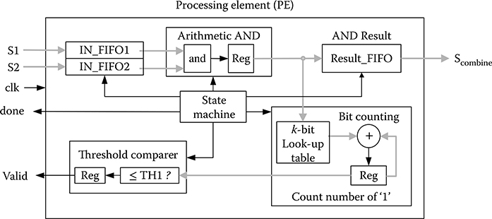
FIGURE 10.8 The architecture of a processing element.

The data width W in the PE is the number of bits that can be executed in each operation. The PE can execute W bits of AND and check W/k bits of “1” at the same time. The number of clock cycles to execute m bit data in each PE is:

{PE}_{cycle} = \frac{m}{W} (1 + \frac{W}{k}) (10.1)

${PE}_{cycle} = \frac{m}{W} (1 + \frac{W}{k}) (10.1)$

10.3.3.2 Data Structure

A custom data structure for the GBC accelerator to provide high efficient combination process is designed. Figure 10.9 shows the data structure of the column pairs in matrix M_S stored in the external memory. The bit “1” in S_ID indicates the columns in matrix M_C that column pair represents. For example, the column pair S_1,2 represents column C1 and column C2 in M_C. The S_ID of S_1,2 is [0000 … 011]. The width of S_ID is Q bits. After storing the S_ID, the bit-vector data of each column pair is stored in the memory. This representation method facilitates the selection of S1 and S2, which reduces data transfer. In the combination Algorithm 1, the accelerator selects two column pairs with at least one common column and one different column in M_C. The column-pair bit vectors are combined only if the conditions are matched. In the example of Figure 10.9, it first reads the S_ID of S_1,2 (S_ID1) and S_1,3 (S_ID2) for checking the conditions. The conditions are checked by using simple AND and XOR gates. The column-pair bit vectors are combined only if both conditions are matched. This saves the time to read the data if the conditions are not matched. If the combined column pair S_combine (S_1,2,3) is valid, the S_ID of S_1,2,3 is equal to S_ID1 OR S_ID2, which is [0000 … 111]. The new S_ID and S_combine are then written to the free memory space.

Images

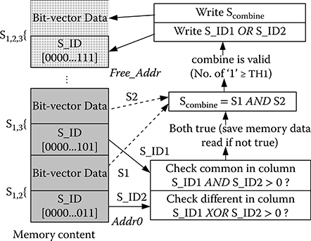
FIGURE 10.9 The data structure of the column pairs in memory.

10.3.4 Experimental Results

In this section, the GBC accelerator on an FPGA is implemented to study the performance by a set of genetic benchmarks. The impact of the PE is studied. A GBC software program is also realized and compared to the GBC accelerator.

10.3.4.1 Genetic Benchmarks

The GBC algorithm is mainly employed for the analysis of large-scale gene microarray data. The gene data is taken as benchmarks to evaluate the performance of the GBC accelerator implemented on FPGA. Six benchmarks of various column-pair matrix size are chosen. The benchmarks are real biological data, which can be downloaded from the National Cancer Institute [42], the Department of Information Technology and Electrical Engineering of ETH Zurich [43] and the National Center for Biotechnology Information [44]. The details of the benchmarks are shown in Table 10.1.

10.3.4.2 Optimization of Geometric Biclustering Accelerator

Internal Structure of PE: Table 10.2 shows the information of the resources used in the GBC accelerator, which is implemented on Xilinx ML605 development platform [45] (using XC6VLX240T-1 FPGA). The number of PEs, data-width, and frequency are scalable depending on the size of the FPGA. Each PE uses three block RAMs for FIFOs. If the architecture and number of PEs are optimized, a higher performance accelerator can be implemented. The impact of the k-bit decoder on the frequency of PEs is shown in Table 10.3. The k-bit decoder counts the number of “1” from k-bit data. The output of the decoder is the number of “1”, which is log₂ k-bits data. From Equation 10.1, when the bit width of the decoder is increased, the number of clock cycles to count the number of “1” decreases. However, this causes the frequency of the PE decreases as shown in Table 10.3. It is because the decoder becomes more complex when k increases. The implementation tool Xilinx Synthesis Tool (Xilinx, San Jose, CA) [46] cannot synthesize the 16-bit decoder because the decoder has 2¹⁶ input combinations, which are not efficiently implemented. As a result, 8-bit decoder is the most time efficient to compute 64-bit data.

Table 10.1 Information of the Six Genetic Benchmarks

Images

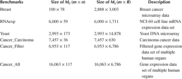
Table 10.2 Information of the Geometric Biclustering Accelerator and Reference C Software Implemented

Images

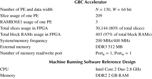
Table 10.3 Optimization of Processing Elements (16-Bit Decoder Cannot Be Synthesized)

k-bit decoder	1	2	4	8	16
PE frequency (MHz)	306	263	269	269	x
Clock cycles (64-bit data)	64	32	16	8	4
Time (64-bit data) (millisecond)	20.9	12.2	5.9	3.0	x

Number of PEs: It is expected that using more PEs can reduce the processing time. Power consumption is a major issue in modern technology. However, it is obvious that more PEs cause higher power consumption, as shown in Figure 10.10. The maximum number of PEs that can be implemented is 130. Therefore, the number of PEs against power and speed of the accelerator should be studied. The power consumption of the accelerator core, which excludes the memory access, is measured by Xilinx XPower Estimator [47]. The average time for combinations of benchmarks is also analyzed. In Figure 10.10, although the power consumed in more PEs is higher, the time to process the GBC algorithm is much lower than less PEs. The energy (power × time) consumed by 130 PEs is the lowest. Therefore, there should be 130 PEs implemented in the accelerator.

Images

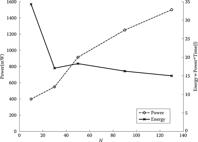
FIGURE 10.10 Power and energy consumption of using a different number of processing elements (maximum 130 processing elements can be implemented).

10.3.4.3 Comparison to Software Reference Design

The hypergraph partitioning method is used to speed up the GBC algorithm in Wang et al. [40]. The time for combining the synthetic benchmark of 100 by 100 matrix is about 2.8 minutes running on the MATLAB environment. The GBC accelerator uses 125 milliseconds to combine this synthetic benchmark, which is over 1350 times faster than Wang et al. [40]. However, it is not a fair comparison because the hypergraph partitioning method is running on an inefficient MATLAB platform. Therefore, the software realization for the GBC algorithm using the highly efficient C language is benchmarked. The algorithm of the GBC software is the same as the GBC accelerator based on Algorithm 1. The software reference design is running on a machine described in Table 10.2. Figure 10.11 shows the comparison between software and accelerator using 130 PEs. On average, the GBC accelerator speeds up the process by four times. In addition, a power meter is utilized to measure the power consumption including memory access power. The software consumes 12.5 W power on average while the accelerator only consumes 7.5 W power when processing. The power reduction is 40%.

10.4 Customizable Very-Large-Scale-Integration Architecture for Compute-Intensive Example

In this section, a FPGA-based customizable SSPPF for neural spiking activity is present. The SSPPF is a kind of adaptive filter that has been applied to the coefficients estimation for neuron models, such as the generalized Laguerre–Volterra model (GLVM). The computation for the SSPPF involves complex matrix/vector calculation. The size of matrix/vector (corresponding to the number of model coefficients) increases exponentially along with the growth of model’s inputs, making the calculation inefficient. This problem is typically compute intensive, which involves calculation on multiple types of data block. Because the data flow throughout the computation cannot be split or divided readily due to the high data dependency in each step, task-level parallelism is not suitable for this case. Nevertheless, hybrid parallel design is adopted, integrating both bit-level and instruction-level parallelism techniques.

Images

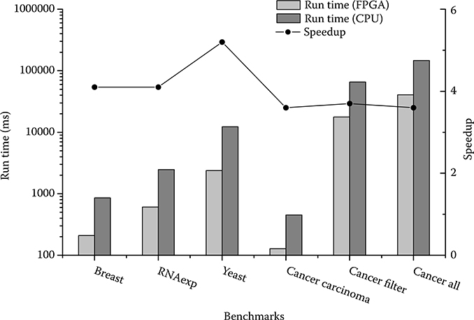
FIGURE 10.11 Work flow of the geometric biclustering algorithm.

10.4.1 Introduction to Generalized Laguerre–Volterra Model and Stochastic State Point Process Filter

As a burgeoning topic in biomedical engineering research, cognitive neural prosthesis requires a silicon-based prosthetic device that can be implanted into the mammalian brain. This device should be capable of performing bidirectional communications between the intact brain regions and bypass the degenerated region [48]. A well-functioning mathematical model has to be established beforehand for effective processing of neural signals. The GLVM, proposed by Song et al. [49], is a data-driven model. It is first applied to predict mammalian hippocampal CA1 neuronal spiking activity based on detected CA3 spike trains, so that the expected neuroprosthetic function can be achieved.

Within the generalized Laguerre–Volterra (GLV) algorithm, the most computation-intensive stage in the overall calculation flow lies in the estimation of the Laguerre coefficients, which has to be done beforehand using the recorded input/output data. Previous silicon-based implementations of the GLVM [50,51], based on the simplified single-input and single-output model, are unable to represent real situation, because a model output is normally affected by multiple inputs of spiking activity. The multi-input, multi-output GLVM was implemented later on an FPGA-based platform [52]. However, the adopted coefficients tracking method is the steepest decent point process filter (SDPPF), which is simple in mathematical expressions but sacrifices certain levels of accuracy, thus being less effective.

The SSPPF is a suitable choice for the aforementioned problem [5]. Derived by Eden et al. [53] based on Bayes rule Chapman–Kolmogorov paradigm and point process observation models, it has been verified to be effective for tracking dynamics of neural receptive fields under various conditions. Chan et al. [54] successfully applied the algorithm to realize the estimation function of the GLVM. A major improvement of SSPPF over SDPPF is the introduction of adaptive learning rate. The adopted learning rate is constant in Li et al. [52]. Although this can simplify the iterative computation procedure, brain activities of the behaving animals can be time variant and subject to stochastic variations. To be more realistic, the learning rate should be updated adaptively using the firing probability computed previously [52] together with the detected model output at present. Up to now, the SSPPF algorithm has been only implemented in software and executed on a desktop setup, resulting in certain limitation in calculation process. Because of the complex computational burden and a potential demand of embedded platform with low power consumption in the future, there is a need of high-performance hardware architecture for this algorithm.

10.4.2 Stochastic State Point Process Filter Algorithm

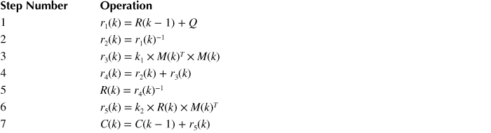
The SSPPF is proposed to adaptively estimate model parameters for point process observations when analyzing neural dynamics [53]. The model of neural firing is defined as a time-varying parameter vector C(k), which is a linear evolution process with Gaussian errors. The C(k) and its covariance matrix R(k) are updated by following recursive equations:

\begin{array}{l} R {(k)}^{- 1} & = {[R (k - 1) + Q]}^{- 1} + [{(\frac{\partial \log P (k)}{\partial C (k)})}^{T} P (k) (\frac{\partial \log P (k)}{\partial C (k)}) \\ - (y (k) - P (k)) \frac{\partial^{2} \log P (k)}{\partial C (k) \partial C {(k)}^{T}}] \end{array} (10.2)

$\begin{array}{l} R {(k)}^{- 1} & = {[R (k - 1) + Q]}^{- 1} + [{(\frac{\partial \log P (k)}{\partial C (k)})}^{T} P (k) (\frac{\partial \log P (k)}{\partial C (k)}) \\ - (y (k) - P (k)) \frac{\partial^{2} \log P (k)}{\partial C (k) \partial C {(k)}^{T}}] \end{array} (10.2)$

C (k) = C (k - 1) + R (k) [{(\frac{\partial \log P (k)}{\partial C (k)})}^{T} (y (k) - P (k))] (10.3)

$C (k) = C (k - 1) + R (k) [{(\frac{\partial \log P (k)}{\partial C (k)})}^{T} (y (k) - P (k))] (10.3)$

where P(k), y(k), and k are the firing probability of spike firing, spike observed, and the discrete time steps, respectively. Applying Equations 10.2 and 10.3 to the GLVM [54], the two equations can be rewritten into the following forms:

R (k) = {[{(R (k - 1) + Q)}^{- 1} + k_{1} M {(k)}^{T} M (k)]}^{- 1} (10.4)

$R (k) = {[{(R (k - 1) + Q)}^{- 1} + k_{1} M {(k)}^{T} M (k)]}^{- 1} (10.4)$

C (k) = C (k - 1) + k_{2} R (k) M {(k)}^{T} (10.5)

$C (k) = C (k - 1) + k_{2} R (k) M {(k)}^{T} (10.5)$

where the vector M(k) is the convolution product between the model inputs/output and the Laguerre basis functions. The k₁ and k₂ can be derived as follows:

k_{1} = α^{2} P (k) + β [y (k) - P (k)] (10.6)

$k_{1} = α^{2} P (k) + β [y (k) - P (k)] (10.6)$

k_{2} = α [y (k) - P (k)] (10.7)

$k_{2} = α [y (k) - P (k)] (10.7)$

α = \frac{1}{\sqrt{2 π} P (k)} \exp [- w {(k)}^{2}] (10.8)

$α = \frac{1}{\sqrt{2 π} P (k)} \exp [- w {(k)}^{2}] (10.8)$

β = \frac{w (k)}{\sqrt{2 π} P (k)} \exp [- w {(k)}^{2}] + \frac{1}{2 π P {(k)}^{2}} \exp [- 2 w {(k)}^{2}] (10.9)

$β = \frac{w (k)}{\sqrt{2 π} P (k)} \exp [- w {(k)}^{2}] + \frac{1}{2 π P {(k)}^{2}} \exp [- 2 w {(k)}^{2}] (10.9)$

The GLVM functions for the calculation of M(k), y(k), P(k), and w(k) were introduced in Chan et al. [54], hence they are not elaborated here. In practice, if the number of parameters in C(k) to estimate is N, R(k) and Q would be an N by N matrix, and M would be a 1 by N vector, while C would be an N by 1 vector.

The SSPPF algorithm is reformed into two major parts. The first part is a collection of a large amount of matrix computation, the most time-consuming and principal aspect of the overall computation. The second part involves intensive arithmetic operations that are difficult for the hardware to implement. Therefore, our architecture of SSPPF is designed to lay a special focus on the calculation stages expressed by Equations 10.4 and 10.5, which has more potential for parallelization. A desktop computer is responsible for the second part and M(k) update, communicating with FPGA in real time.

10.4.3 Architecture Design

10.4.3.1 Parallelism Exploration for the Stochastic State Point Process Filter Algorithm

First, the parallel design techniques should be considered comprehensively to realize an efficient architecture. The overall computation flow is decomposed into seven steps, which are presented in Table 10.4. It is straightforward to see that the computation flow is difficult to be separated into subtasks that can be performed in parallel, as data dependency exists between consecutive steps. These tasks need to be carried out in a sequential way. In addition, the data involved in SSPPF is either matrix or vector; data partitioning and assembling method is not that appropriate when certain operations like matrix inversion are performed, which would make the overall complexity high. Therefore, neither task-level nor data-level parallelism is optimized to utilize.

Table 10.4 Steps to Finish One Iteration of Stochastic State Point Process Filter (N: Vector/Matrix Size)

Images

Exploiting bit-level and instruction-level parallelism makes sense for the architecture of SSPPF. Bit-level exploration implies increasing the data width, by concatenating multiple operands to form a vector and processing at one time. This method is also referred to as vector processing [55]. The data organizational format in SSPPF algorithm is suitable to be handled in a vector manner, and the intrinsic properties of VLSI/FPGA facilitate this technique. First, the on-chip memory blocks (block RAMs) are customizable in data width, because multiple block RAMs can be cascaded to cache wide words. By this, a vector of data in one memory address is stored and accessed, not requiring extra instructions, which reduces power consumption. Second, vector processing demands certain data alignment to meet specific requirements of the underlying algorithm. FPGAs provide the design freedom to create a custom alignment unit, which would further improve performance and power consumption [56]. Finally, the reconfigurability of an FPGA allows us to explore multiple degrees of vectorization and choose the optimal one to meet the area and throughput constraints [55].

Instruction-level parallel design needs to execute multiple instructions in parallel. Pipelining is an efficient architecture mechanism that exploits instruction-level parallelism at run time [57]. It can be viewed as a form of parallelism where a process is divided into a set of stages, all of the stages run concurrently, and the output of each stage acts as the input to the next one. The goal is to hide the latency of operations in parallel, increase system throughput by overlapping (in time) the execution of the stages, and maximize the instruction efficiency [28,57].

10.4.3.2 Architecture for Stochastic State Point Process Filter

The parallel VLSI architecture for SSPPF is constructed taking into consideration the discussed techniques. The data representation adopted is single precision floating-point format in the IEEE-754 standard, so each data is represented by 32 bits. Unlike most hardware designs [52,58], the matrix size can be dynamically changed to be arbitrary in each updating iteration in this architecture, without preconfiguration. The size of matrix/vector is only limited by on-chip memory resource. The architecture is also scalable in degree of parallelism, because the computing units are capable of concatenating to increase the degree of vector processing.

Images

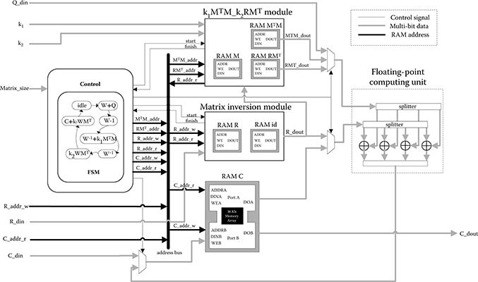
FIGURE 10.12 Overall architecture of stochastic state point process filter.

Figure 10.12 shows the overall architecture for SSPPF. The top layer module implements two submodules according to principal steps in SSPPF calculation: the computation of k₁M(k)^TM(k) and k₂R(k)M(k)^T is conducted in k₁ M^TM_k₂RM^T module; the inversion of R(k) is performed by matrix inversion module. Vectors and matrices involved are stored in block RAMs some of which are arranged to true dual-port mode to enable concurrent reading and writing.

At the top and matrix inversion module, vector processing method is employed: a vector of four floating-point data constitutes the basic operand, while a computing unit consists of four floating-point operators. The intrinsic FPGA parallelism can be further explored by combining more computing units in parallel, with data-width for operation and storage increased accordingly. Operations are performed in horizontal sweep fashion, which is to process multiple elements of a row in parallel until the entire row is scanned.

The matrix inversion module is shown in Figure 10.13, which is based on the Gauss–Jordan elimination algorithm with partial pivoting. Given an N by N square matrix A, the inversion process begins by building an augmented matrix with the size N by 2N: [AI]. The identity matrix I is on the right side of A. Row operations are then performed iteratively to transform [AI] into [IA⁻¹]. Two sets of operators and RAMs are needed for original and identity matrix simultaneously. The calculations in two time-consuming phases—normalization and elimination—are fully pipelined. Elimination module is in charge of these two calculations as shown in Figure 10.14. The pivot row normalization step is realized by multiplying the pivot’s reciprocal calculated in advance, by each row element. Two block RAMs are set to synchronize multiple operand flows in the computing units: one to cache a normalized pivot row and another to cache all elements in the column where the pivot is located. The control logic continuously generates address signals to various RAMs for reading and writing. The true dual-port RAMs facilitate the pipelining operation through concurrent operations: reading vectors of data from one port and receiving results in another port.

Images

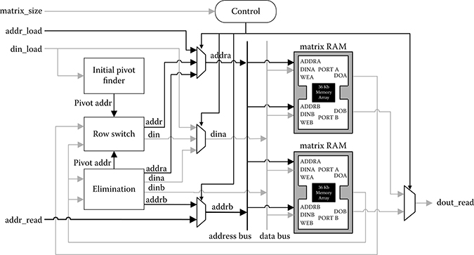
FIGURE 10.13 Matrix inversion module. Maximal parallelism is explored in this module by vector processing and pipelining.

Images

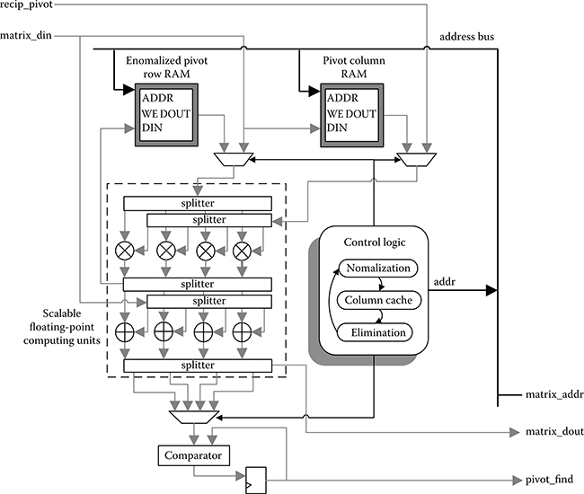
FIGURE 10.14 Elimination module is the focus of computation, because the elimination phase is most time-consuming throughout the inversion process. Indeed, two sets of computing units are implemented for original and identity matrix, but only one set is presented in this figure.

To achieve efficient pivot location, a comparator is set as the last node in the computing pipeline, directly receiving data flow from adder outputs. Pivot search is thus performed with only one extra clock in general. The found pivot row address is output for next-round row interchange when the elimination process is done. In this module, both bit-level and instruction-level parallelism are fully achieved through deep pipelining and vector processing.

In the k₁M^TM_k₂RM^T module, the memory of vector M(k) together with floating-point operators is shared by two distinct calculations, as shown in Figure 10.15. Only a minimum number of operators are implemented in this module, because the two involved computations are not bottlenecks affecting the overall performance, which only consume a small portion of the total calculation time.

The approximated number of clock cycles in each round of C(k) update is estimated in Equation 10.10. The D_P denotes the parallel degree (it is four in the current design), and N denotes matrix/vector size. In this estimation, both the latency of operator intellectual property cores and the control signal overheads are overlooked; each would be fairly trivial when the size N increases.

(2 N^{2} + 28 N) ⌈ \frac{N}{D_{P}} ⌉ + 4 N^{2} + N (10.10)

$(2 N^{2} + 28 N) ⌈ \frac{N}{D_{P}} ⌉ + 4 N^{2} + N (10.10)$

Images

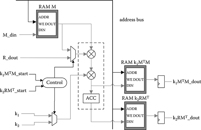
FIGURE 10.15 k₁M^TM_k₂RM^T module, where the calculation of k₁M(k)^TM(k) and k₂R(k)M(k)^T are performed.

10.4.4 Experimental Results

The architecture is synthesized, placed, and routed on a Xilinx Virtex-6 FPGA (XC6VLX240T-1). The resources occupied by the whole architecture and the main modules are summarized in Table 10.5. The upper limit of matrix/vector size N is set to 256 under consideration of available on-chip memory. The resource usage is rather small except for block RAMs.

The functionality of the SSPPF architecture needs to be verified, so two sets of synthetic experimental data are selected as the initial input into the hardware. The size of vector C(k) is set to be 49 and 139 in experiments, which accounts for the coefficients to estimate in a multi-input single-output model, and under two specific conditions: (1) only second-order self-kernel is applied, (2) both self-kernel and cross kernel in second order are applied. All kernels (besides the 0th) have five inputs, and the number of Laguerre basis functions L is set at 3 [52,59]. Meanwhile, the Laguerre coefficients estimation in MATLAB description of SSPPF algorithm is realized with a double precision floating-point format as a reference. The estimated vector C(k) of one iteration calculated by two platforms is shown in Figure 10.16. The results seem to be the same, and error analysis needs to be carried out to identify the achievable accuracy.

In error analysis, a comparison is made between the results achieved by FPGA design and MATLAB realization in double precision. Initial input coefficient vector and covariance matrix are randomly generated. Absolute maximum value of k₁ and k₂ under worst conditions is chosen to evaluate possible maximum error. There are 100 independent experiments performed to update C(k) and calculate the average mean error (ME) and mean squared error (MSE) of FPGA implementation results in each SSPPF iteration. The ME and MSE are computed with Equations 10.11 and 10.12 (the i is the element index in C(k)), respectively (Figure 10.17). Although both values increase as size N grows because of the error cumulation, the MSE for N = 250 remains under 2 × 10⁻⁸.

ME = \frac{1}{100} \sum_{k = 1}^{100} [\frac{1}{N} \sum_{i = 1}^{N} | C_{FPGA} (k) (i) - C_{MATLAB} (k) (i) |] (10.11)

$ME = \frac{1}{100} \sum_{k = 1}^{100} [\frac{1}{N} \sum_{i = 1}^{N} | C_{FPGA} (k) (i) - C_{MATLAB} (k) (i) |] (10.11)$

Table 10.5 Resource Utilization of Architecture Design

	k₁M^TM_k₂RM^T Module	Matrix Inversion Module	Overall Design
Slice LUTs	2344 (1%)	12,068 (8%)	16,667 (11%)
Slice registers	2905 (1%)	14,139 (4%)	19,035 (6%)
RAMB36E1	57 (13%)	118 (28%)	176 (42%)
RAMB18E1	2 (1%)	1 (1%)	3 (1%)
Maximum frequency	261.575 MHz	220.653 MHz	208.247 MHz

Images

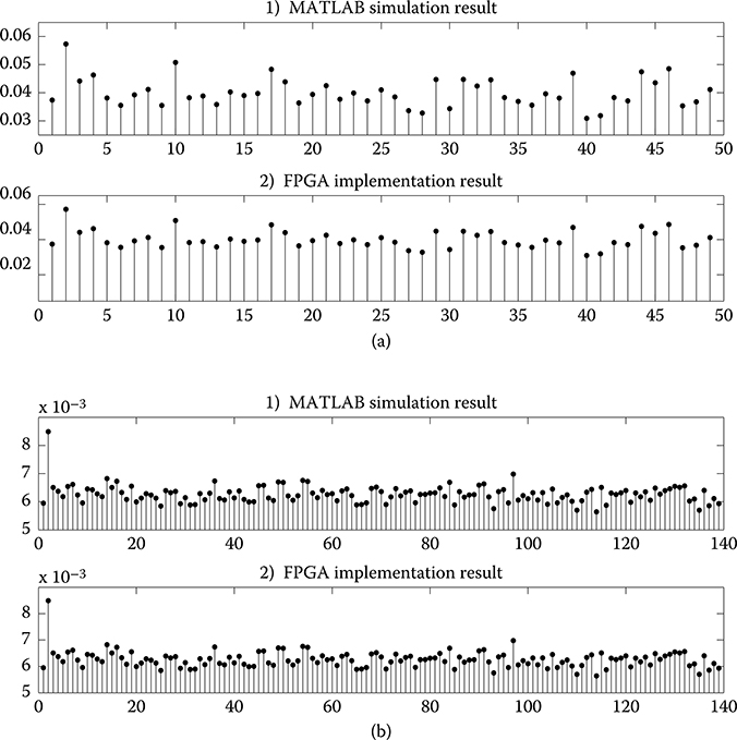
FIGURE 10.16 Result comparison between field-programmable gate array implementation and MATLAB simulation. (a) The upper part is the result for N = 49, and (b) the lower part is the result for N = 139.

ME = \frac{1}{100} \sum_{k = 1}^{100} [\frac{1}{N} \sum_{i = 1}^{N} {(C_{FPGA} (k) (i) - C_{MATLAB} (k) (i))}^{2}] (10.12)

$ME = \frac{1}{100} \sum_{k = 1}^{100} [\frac{1}{N} \sum_{i = 1}^{N} {(C_{FPGA} (k) (i) - C_{MATLAB} (k) (i))}^{2}] (10.12)$

In a performance evaluation for execution speed, the hardware architecture is compared with software running on a commercial CPU platform. The software implementation of SSPPF algorithm in C language has been benchmarked. Configuration of the software platform is given in Table 10.6. Different datasets with the number of coefficients ranging from 50 to 250 are executed on two platforms. The FPGA architecture is driven by its possible maximum frequency clock in the evaluation.

The bar graph in Figure 10.18 illustrates the execution-time comparison between two platforms for various matrix sizes. The FPGA-based hardware platform can achieve up to seven times speedup compared to the software implementation in calculation efficiency. Considering the degree of vector processing in this design is only four, the speedup would be much more significant by an exploration of higher degree of parallelism in the future work.

Images

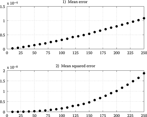
FIGURE 10.17 Mean error and mean squared error of the field-programmable gate array results with different matrix size N.

Table 10.6 Software Execution Platform

CPU	Intel Core^(TM) i5-250M @ 2.50GHz
RAM	4GB
Compiler	Visual Studio 2010

10.5 Conclusions

The VLSI technology plays an essential role in HPC field, and is widely applied in modern bioinformatics and biomedical engineering. There has been a transfer of research focus from conventional processors to parallel hardware architecture, to explore more efficient computation.

In this chapter, we have discussed the immense potential of VLSI architecture in bioinformatic and biomedical applications. Two grouping methods of the parallel computing problems are provided from different perspectives, together with several design techniques. Two high-performance VLSI architectures in applications of bioinformatics and biomedical engineering are presented. These two applications belong to data-intensive and compute-intensive problems, which are representatives in parallel architecture design. Multiple parallel levels and design techniques are explored efficiently.

Images

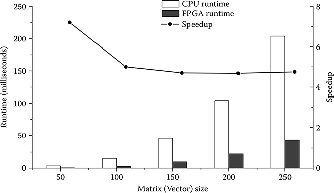
FIGURE 10.18 Execution time comparison between hardware and software platform, with different matrix size N.

The first design is a scalable FPGA-based accelerator for a GBC algorithm. By exploring hybrid parallelism, it has reached a considerable acceleration as well as low energy consumption, when compared with a software implementation on a CPU platform. The second design is a hardware architecture for the SSPPF, which is an adaptive filter to estimate neuron model coefficients in neural spiking activity. Bit-level and instruction-level parallel techniques are employed. This architecture is scalable in terms of both matrix size and degree of parallelism. Experimental results show that it is possible to outperform software implementation by making full use of the intrinsic parallel property of VLSIs.

In the future, more efficient VLSI architectures should be explored. In current GBC accelerator, the performance is restricted by the limited memory bandwidth, because data-intensive applications demand a high throughput. More powerful platforms equipped with large-capacity chip and high-bandwidth external memory would be utilized to break the bottleneck of PE number and data transfer throughput. The current SSPPF architecture only adopts a parallelism degree of four, so there is still a large space to explore for a deeper bit-level parallelism. Besides, more effective design techniques in different parallelism levels should also be considered, to reduce power consumption and enhance the computation efficiency.

References

1. N. M. Luscombe, D. Greenbaum, and M. Gerstein, “What is bioinformatics? An introduction and overview,” Department of Molecular Biophysics and Biochemistry, Yale University, New Haven, CT, Tech. Rep., 2001.

2. D. A. Benson, I. Karsch-Mizrachi, D. J. Lipman, J. Ostell, and D. L. Wheeler, “Genbank,” Nucleic Acids Research, 36(suppl 1): D25–D30, 2008.

3. M. Burrows and D. J. Wheeler, “A block-sorting lossless data compression algorithm,” Tech. Rep. 124, 1994.

4. Y. Xin, B. Liu, B. Min, W. X. Y. Li, R. C. C. Cheung, A. S. Fong, and T. F. Chan, “Parallel architecture for DNA sequence inexact matching with Burrows-Wheeler Transform,” Microelectronics Journal, 44(8): 670–682, 2013.

5. H. Li and R. Durbin, “Fast and accurate short read alignment with Burrows-Wheeler transform,” Bioinformatics, 25(14): 1754–1760, July 2009.

6. B. Langmead and S. L. Salzberg, “Fast gapped-read alignment with Bowtie 2,” Nature Methods, 9(4): 357–359, March 2012.

7. G. Christine and K. Arthur, “Imaging calcium in neurons,” Neuron, 73(5): 862–885, 2012.

8. C. Eliasmith and C. H. Anderson, Neural Engineering (Computational Neuroscience Series): Computational, Representation, and Dynamics in Neurobiological Systems. Cambridge, MA: MIT Press, 2002.

9. L. Paninski, J. Pillow, and J. Lewi, “Statistical models for neural encoding, decoding, and optimal stimulus design,” in Computational Neuroscience: Progress in Brain Research, ed. P. Cisek, T. Drew, and J. F. Kalaska. Amsterdam, the Netherlands: Elsevier, 2006.

10. J. Enderle, J. Bronzino, and S. Blanchard, Introduction to Biomedical Engineering, ser. Academic Press Series in Biomedical Engineering. Burlington, MA: Elsevier Academic Press, 2005.

11. L. Hasan, Z. Al-Ars, and S. Vassiliadis, “Hardware acceleration of sequence alignment algorithms-an overview,” Design Technology of Integrated Systems in Nanoscale Era, pp. 92–97. DTIS International Conference on, Rabat, Morocco, September 2007.

12. X. Gan, A. Liew, and H. Yan, “Discovering biclusters in gene expression data based on high-dimensional linear geometries,” BMC Bioinformatics, 9(1): 1–15, 2008.

13. M. Nei, “Phylogenetic analysis in molecular evolutionary genetics,” Annual Review of Genetics, 30(1), 371–403, 1996.

14. C. A. Stewart, R. Z. Roskies, and S. Subramaniam, “Opportunities for biomedical research and the NIH through high performance computing and data management,” Indiana University, Tech. Rep., 2003.

15. National Center for Biological Information, “Genbank Statistics.” Available at http://www.ncbi.nlm.nih.gov/genbank/statistics, accessed September 15, 2013.

16. “UniProtKB/TrEMBL Protein Database Release Statistics.” Available at http://www.ebi.ac.uk/uniprot/TrEMBLstats, accessed September 15, 2013.

17. R. K. Weinstein and R. H. Lee, “Architectures for high-performance FPGA implementations of neural models,” Journal of Neural Engineering, 3(1): 21, 2006.

18. E. Graas, E. Brown, and R. Lee, “An FPGA-based approach to high-speed simulation of conductance-based neuron models,” Neuroinformatics, 2(4): 417–435, 2004.

19. M. Gschwind, H. P. Hofstee, B. Flachs, M. Hopkin, Y. Watanabe, and T. Yamazaki, “Synergistic processing in cell’s multicore architecture,” Micro, IEEE, 26(2): 10–24, 2006.

20. B. Liu, C. W. Yu, D. Z. Wang, R. C. C. Cheung, and H. Yan, “Design exploration of geometric biclustering for microarray data analysis in data mining,” Parallel and Distributed Systems, IEEE Transactions on, PP(99): 1, 2013.

21. “San Diego Supercomputer Center.” Available at http://www.sdsc.edu/, accessed September 15, 2013.

22. “Pittsburgh Supercomputing Center.” Available at http://www.psc.edu/, accessed September 15, 2013.

23. “Accelerating high-performance computing with FPGAs,” Altera, Tech. Rep., 10, 2007.

24. H. Esmaeilzadeh, E. Blem, R. St. Amant, K. Sankaralingam, and D. Burger, “Dark silicon and the end of multicore scaling,” Micro, IEEE, 32(3): 122–134, 2012.

25. “High performance computing using FPGAs,” Xilinx, Tech. Rep., 9, 2010.

26. B. Schmidt, Bioinformatics: High Performance Parallel Computer Architectures. Boca Raton: FL: CRC Press, 2010.

27. B. Mackin and N. Woods. “FPGA Acceleration in HPC: A Case Study in Financial Analytics.” XtremeData Inc. White Paper, 2006.

28. M. Walton, O. Ahmed, G. Grewal, and S. Areibi, “An empirical investigation on system and statement level parallelism strategies for accelerating scatter search using Handel-C and Impulse-C,” VLSI Des., 2012: 5:5–5:5, January 2012.

29. An Xtremedata, “Scalable FPGA-Based Computing Accelerates C Applications.” The Free Library, 2006.

30. F. I. Cheema, Zain-ul-Abdin, and B. Svensson, “A design methodology for resource to performance tradeoff adjustment in FPGAs,” in Proceedings of the 7th FPGAworld Conference, ser. FPGAworld ’10, 14–19. New York: ACM, 2010.

31. S. Scott and F. Alessandro, “Where’s the beef? Why FPGAs are so fast,” Microsoft Research, Tech. Rep., September 2008.

32. K. Asanovic, R. Bodik, B. C. Catanzaro, J. J. Gebis, P. Husbands, K. Keutzer, D. A. Patterson, W. L. Plishker, J. Shalf, S. W. Williams, and K. A. Yelick, “The landscape of parallel computing research: A view from Berkeley”, EECS Department, University of California, Berkeley, Tech. Rep., December 2006.

33. I. Gorton, P. Greenfield, A. Szalay, and R. Williams, “Data-intensive computing in the 21st century,” Computer, 41(4): 30–32, 2008.

34. B. Furht and A. Escalante, Handbook of Cloud Computing. New York: Springer, 2010.

35. T. Bunker and S. Swanson, “Latency-optimized networks for clustering FPGAs,” in Field-Programmable Custom Computing Machines (FCCM), pp. 129–136, 2013 IEEE 21st Annual International Symposium, Seattle, WA, 2013.

36. T. R. Golub, D. K. Slonim, P. Tamayo, C. Huard, M. Gaasenbeek, J. P. Mesirov, H. Coller et al., “Molecular classification of cancer: Class discovery and class prediction by gene expression monitoring,” Science, 286(5439): 531–537, 1999.

37. X. Gan, A. W. C. Liew, and H. Yan, “Discovering biclusters in gene expression data based on high-dimensional linear geometries,” BMC Bioinformatics, 9(1): 209, 2008.

38. S. Liu, Y. Chen, M. Yang, and R. Ding, “Bicluster Algorithm and used in market analysis,” in Second International Workshop on Knowledge Discovery and Data Mining, pp. 504–507, Moscow, 2009.

39. H. Zhao, A. W. C. Liew, X. Xie, and H. Yan, “A new geometric biclustering algorithm based on the Hough transform for analysis of large-scale microarray data,” Journal of Theoretical Biology, 251(3): 264–274, 2008.

40. D. Z. Wang and H. Yan, “Geometric biclustering analysis of DNA microarray data based on hypergraph partitioning,” in IDASB Workshop on BIBM2010, pp. 246–251, Hong Kong, People’s Republic of China, 2010.

41. M. Gokhale, J. Cohen, A. Yoo, W. Miller, A. Jacob, C. Ulmer, and R. Pearce, “Hardware technologies for high-performance data-intensive computing,” Computer, 41(4): 60–68, 2008.

42. Cellminer Database. “NCI-60 Analysis Tools.” Available at http://discover.nci.nih.gov/cellminer, accessed September 15, 2013.

43. Department of Information Technology and Electrical Engineering of ETH Zurich. Available at http://www.tik.ee.ethz.ch/~sop/bimax/SupplementaryMaterial/Datasets/BiologicalValidation, accessed September 15, 2013.

44. National Center for Biotechnology Information. Available at http://www.ncbi.nlm.nih.gov/guide, accessed September 15, 2013.

45. Xilinx, Inc., “Getting Started with the Xilinx Virtex-6 FPGA ML605 Evaluation Kit, UG533 (v1.5),” 2011. Available at http://www.xilinx.com/support/documentation/boards_and_kits/ug533.pdf, accessed September 15, 2013.

46. Xilinx, Inc., “XST User Guide for Virtex-6 and Spartan-6 Devices, UG687 (v12.3),” 2010. Available at http://www.xilinx.com/support/documentation/swmanuals/xilinx124/xstv6s6.pdf, accessed September 15, 2013.

47. Xilinx, Inc., “XPower Estimator User Guide,” 2011. Available at http://www.xilinx.com/support/documentation/userguides/ug440.pdf, accessed September 15, 2013.

48. T. W. Berger, D. Song, R. H. M. Chan, and V. Z. Marmarelis, “The neurobiological basis of cognition: Identification by multi-input, multioutput nonlinear dynamic modeling,” Proceedings of the IEEE, 98(3), 356–374, March 2010.

49. D. Song, R. H. M. Chan, V. Z. Marmarelis, R. E. Hampson, S. A. Deadwyler, and T. W. Berger, “Nonlinear dynamic modeling of spike train transformations for hippocampal-cortical prostheses,” IEEE Transactions on Biomedical Engineering, 54(6): 1053–1066, June 2007.

50. T. W. Berger, A. Ahuja, S. H. Courellis, S. A. Deadwyler, G. Erinjippurath, G. A. Gerhardt, G. Gholmieh et al., “Restoring lost cognitive function,” Engineering in Medicine and Biology Magazine, IEEE, 24(5): 30–14, September–October 2005.

51. M. C. Hsiao, C. H. Chan, V. Srinivasan, A. Ahuja, G. Erinjippurath, T. Zanos, G. Gholmieh et al., “VLSI implementation of a nonlinear neuronal model: A ‘Neural Prosthesis’ to restore Hippocampal Trisynaptic Dynamics,” in Engineering in Medicine and Biology Society, 2006. EMBS ’06. 28th Annual International Conference of the IEEE, pp. 4396–4399, New York, NY, August 30, 2006–September 3, 2006.

52. W. X. Y. Li, R. H. M. Chan, W. Zhang, R. C. C. Cheung, D. Song, and T. W. Berger, “High-performance and scalable system architecture for the real-time estimation of generalized Laguerre-Volterra MIMO model from neural population spiking activity,” IEEE Journal on Emerging and Selected Topics in Circuits and Systems, 1(4): 489–501, December 2011.

53. U. T. Eden, L. M. Frank, R. Barbieri, V. Solo, and E. N. Brown, “Dynamic analysis of neural encoding by point process adaptive filtering,” Neural Computation, 16(5): 971–998, May 2004.

54. R. H. M. Chan, D. Song, and T. W. Berger, “Nonstationary modeling of neural population dynamics,” in Engineering in Medicine and Biology Society, 2009. EMBC 2009. Annual International Conference of the IEEE, pp. 4559–4562, September 2009.

55. X. Chen and V. Akella, “Exploiting data-level parallelism for energy-efficient implementation of LDPC decoders and DCT on an FPGA,” ACM Trans. Reconfigurable Technology Systems, 4(4): 37:1–37:17, December 2011.

56. J. Oliver and V. Akella, “Improving DSP performance with a small amount of field programmable logic,” in Field Programmable Logic and Application, ser. Lecture Notes in Computer Science, P. Cheung and G. Constantinides, Eds. New York: Springer Berlin Heidelberg, 2003, 2778: 520–532.

57. Z. Guo, W. Najjar, F. Vahid, and K. Vissers, “A quantitative analysis of the speedup factors of FPGAs over processors,” in Proceedings of the 2004 ACM/SIGDA 12th international symposium on Field programmable gate arrays, ser. FPGA ’04. pp. 162–170, New York: ACM, 2004.

58. X. Zhu, R. Jiang, Y. Chen, S. Hu, and D. Wang, “FPGA implementation of Kalman filter for neural ensemble decoding of rat’s motor cortex,” Neurocomputing, 74(17): 2906–2913, 2011.

59. D. Song, R. H. M. Chan, V. Z. Marmarelis, R. E. Hampson, S. A. Deadwyler, and T. W. Berger, “Nonlinear modeling of neural population dynamics for hippocampal prostheses,” Neural Networks, 22: 1340–1351, 2009.

..................Content has been hidden....................

You can't read the all page of ebook, please click here login for view all page.

Table of Contents for
10 High-Performance and Customizable Bioinformatic and Biomedical Very-Large-Scale-Integration Architectures