
18 Ultra-Low-Power Audio Communication System for Full Implantable Cochlear Implant Application
Yannick Vaiarello and Jonathan Laudanski
Contents
18.2.1 Outer and Middle Ear: From Acoustics to Mechanics Waves
18.2.2 Inner Ear: Transducing Hydraulic Waves into Electric Signals
18.3 Pathologies of Hearing and Hearing Prothesis
18.3.1 Middle Ear Pathologies and Middle Ear Implant
18.3.2 Inner Ear Pathology and Cochlear Implants
18.3.3 Future Solution: Full Implantable Device
18.4.1 Physical Dimensions and Consumption
18.4.2.2 Frequency and Link Budget
18.6 Wireless Microphone Design
18.6.3 Analog to Time Converter
18.7 Implementation and Experimental Results
In memory of Jonathan, who passed away in an accident on May 11, 2014.
18.1 Introduction
The ear is a formidable organ capable of encoding sensory information over an incredible range of intensities of more than 12 orders of magnitude. With it, our hearing function can easily track the voice of someone speaking amidst a room full of conversations (the well-known cocktail-party effect). The ear is a fast entry point to our brain and provides a very good temporal accuracy. For instance, we are able to detect a gap of a few milliseconds or differences in timing of a few microseconds between our two ears. In comparison, our retina provides to the visual system with a relatively slow input that does not even allow us to perceive the 50-Hz flickering of a light bulb.
After describing how the complex apparel of the inner ear transforms pressure waves into nerve signals, we expose the different pathologies of the ear, their functional effect, and the social impacts. We focus then on the implanted medical devices alleviating the profound deafness, particularly the cochlear implant. In the prospect of designing a future fully implantable system, we describe in detail the only external device of this system: the microphone.
18.2 Ear and Hearing Brain
18.2.1 Outer and Middle Ear: From Acoustics to Mechanics Waves
Sound enters into the ears as an acoustic wave through the air before entering through the pinna, the concha, and the external auditory meatus as displayed in Figure 18.1. This succession of elements constitutes the outer ear, which conveys acoustical waves to the tympanic membrane in the middle ear. The pinna plays an important role in amplifying and shaping the sound spectrum: it creates troughs and peaks at certain frequency [1,2]. This directional spectral amplification is critical for localizing sounds vertically and to disambiguate back from front horizontally [2].
The middle ear is composed of the tympanic membrane and three bones: the malleus, the incus, and the stapes. Its main role is the transformation of acoustical waves into hydrodynamic wave inside the cochlea (see Figure 18.1) [3]. This requires a complex energy efficient impedance matching. The main amplification is produced by collecting pressure over the large surface of the tympanic membrane and transmitting it into the small oval window. Without it, most sound energy would be reflected by the fluid surface, and only a small percent of this energy would be transmitted.
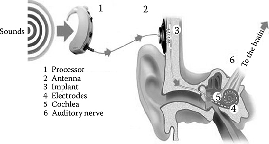
FIGURE 18.1 Cochlear implant system.
A second amplification is produced by a lever effect. The malleus is longer than the incus by around 20% and because both are connected by elastic cartilage articulation, a small gain is produced. The elastic properties of the articulations render the gain frequency dependent [3]. Furthermore, the transmission of the mechanic energy via the ossicular chain allows a second important role for the middle ear: the protection of the inner ear against loud sounds. The stapedian muscle connects to the incus and contracts when sound level is over 70–85 dB [4,5]. This mechanism, called stapedius reflex, produces a change in the ossicular chain’s impedance and can reduce its gain by up to 15–20 dB for frequencies in the range 500 Hz to 1.5 kHz [5,6].
18.2.2 Inner Ear: Transducing Hydraulic Waves into Electric Signals
The last bone of the ossicular chain, the stapes, transmits pressure changes through the oval window to the inner fluid of the cochlea. This snail-shaped organ is embedded deeply in the temporal bone and composed of three spiraling ducts of about 35 mm. These ducts are separated by membranes that are oscillating in response to the pressure waves produced by the ossicles. More specifically, a travelling wave is initiated on the basilar membrane on which lies the organ of Corti. The organ of Corti contains two types of hair cells: the inner hair cells (IHCs), which are transducers, and the outer hair cells (OHC), which act as amplifiers of the basilar membrane movement. Depolarization of the IHCs release neurotransmitter, which triggers action potentials in the auditory nerve fibers.
The motion of the stapes initiates a travelling wave in the cochlear duct. This wave can be observed on both membranes and was originally recorded stroboscopically by von Bekesy [7]. Because the basilar membrane has a varying mass and stiffness along its length, at each position the membrane possesses a specific resonant frequency, called the characteristic frequency. The cochlea thus performs a time–frequency decomposition of the hydrodynamic waveform. The time–frequency decomposition provides an accurate representation of the sound energy contained in each frequency band. This mapping of frequency to cochlear position is called the tonotopy and is a major factor used when restoring hearing using cochlear implants.
18.3 Pathologies of Hearing and Hearing Prothesis
The transformation of acoustical waves into auditory nerve discharges is a sequence of complex and intricate stages. At each of these stages, the possibility of a malfunctioning exists. Around 15% of teenagers suffer from hearing loss [8], a prevalence rate that increases to 63% for adults older than 70 [9]. For most cases, the hearing problems are linked to the aging of the auditory system. The progressive loss of OHC produces sensorineural hearing loss, a condition characterized by reduced audibility (i.e., increased threshold of hearing), reduced frequency selectivity (i.e., increased bandwidth of the basilar membrane resonance), and abnormal loudness growth. No treatment exists to restore fully the hearing function and hearing impairment is alleviated by the use of hearing aids. Hearing aids are complex amplifying devices that help perceive low-level sounds and avoid the sensation of abnormal loudness growth. This chapter deals with microphone for implantable devices prescribed in the case of more severe hearing problems.
18.3.1 Middle Ear Pathologies and Middle Ear Implant
There are many origins of middle ear pathologies [10]. In the case of ossicular chain malformations, or otospongiosis [11] or ossification of the articulations after repeated otitis media [12], an important decrease in audibility is observed resulting from the loss of the sound transmission. At least two devices are available depending on whether the inner ear is also affected. Replacement of one of the ossicles by an implanted device can be performed [13,14]. In the case of putative inner ear malfunction on the same side as middle ear pathology, the treatment is usually to reroute the sound to the other ear using bone-anchored hearing system [15,16].
18.3.2 Inner Ear Pathology and Cochlear Implants
Irreversible loss or malfunctioning of IHCs results in the impossibility to treat deafness by amplification of vibrations irrespective of whether these are hydrodynamic or bony vibrations. Whether the pathologies are of genetic origin (connexin deficiency [17], Jervell and Lange-Nielsen’s syndrome, Meniere’s syndrome, etc. [18]), traumatic (loud sound exposure, temporal bone fracture), or results from an extended medical history (aging, ototoxic treatment, recurrent otitis media, etc.), IHC impairment produces profound (70 dB < loss < 90 dB) to severe hearing loss (>90 dB). However, the loss of the IHCs does not imply a pathological state for the auditory nerve and fibers may be present and fully functional. Indeed, the degeneration of nerve auditory fibers is progressive over a timescale of a few years after IHC loss.
The cochlear implant is an active device with no implanted battery (unlike pace-making devices), which obtains both its energy and stimulating command from an outside “behind-the-hear” processor. A high-frequency magnetic transcutaneous communication link transmits a sparse representation of the sound energy present in different frequency bands. The implant then stimulates sequentially electrodes disposed along the length of the cochlea. By using the tonotopic organization of the cochlea, the implant activates the auditory nerve fibers and produces a coarse grained spectro-temporal representation of sound. The current Neurelec device has a diameter of 28 mm and a height of 4–5.5 mm. The electrode array inserted into the cochlea has 20 channels. The microphone has a dynamic range of 75 dB and a sampling frequency of 16.7 kHz. Cochlear implantation offers now speech understanding in quiet environments to implanted users, with major clinical benefits in terms of social interactions and quality of life [19].
18.3.3 Future Solution: Full Implantable Device
The new device will be fully implanted. Thus, with this system, the processor and the microphones are located with the neurostimulation circuit on the patient’s head. To power this system, a rechargeable battery is inserted under the skin of the patient. The importance of the detailed module in this chapter occurs in the case of a malfunction of the implanted microphone. In order not to operate on the patient again, a microphone with radio frequency (RF) link to communicate with the implant will be provided while being as unobtrusive as possible [20]. This module, shown in Figure 18.2, will be placed in the ear canal of the patient to make it almost invisible.
18.4 Specifications
18.4.1 Physical Dimensions and Consumption
The integration of the system including a microphone [21], battery [22], a transmitting antenna, and a printed circuit board (PCB) containing an integrated circuit dedicated to the application shall not exceed a volume of 6 mm (diameter) by 10 mm (height).
This constraint passed on the microphone or battery requires the use of button cells battery (A10), which is the volume occupied by 5.8 mm to 3.6 mm (diameter to height) for a nominal capacity of 95 mAh. For patient comfort, it is necessary that the product has a lifetime of about 3 days with 10 hours of use per day. This constraint allows us to determine the average power consumption of the circuit should not exceed 3.2 mA at 1.2 V.
18.4.2 Radio Frequency Link
18.4.2.1 Propagation Channel
The system will incorporate a communication from the outside to the inside of the human body. The propagation channel is composed of skin, cartilage, and fat. It connects the transmitter module placed in the ear canal and the receiver, implanted, located at the temple against the skull.
18.4.2.2 Frequency and Link Budget
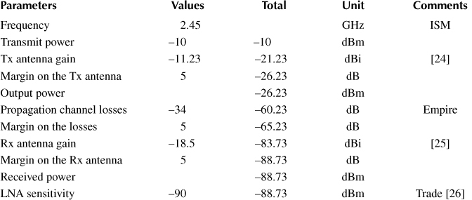
Carrier frequency choice is a compromise between physical size and attenuation in the propagation channel. Indeed, the higher the frequency, the higher its integration will be easy. Nevertheless, the higher the frequency, the higher the attenuation in this environment will be important. Therefore, and considering only the band of free with permission of audio transfer, our choice fell on the 2.45 GHz Industrial, Scientific, and Medical (ISM) (radio spectrum) standard [23]. Figure 18.3 shows the simulation of the propagation channel has 2.45 GHz by considering different electromagnetic characteristics of each tissue (Table 18.1) on the Empire tools. We notice in this figure that the attenuation at the location of the implant is about 34 dB. Finally, Table 18.2 shows the link budget of our application made by these results and a literature review and showing that the radio link is possible.
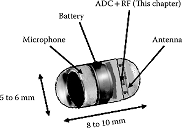
FIGURE 18.2 Description of the module.
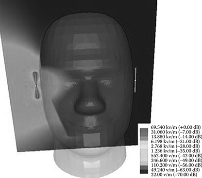
FIGURE 18.3 Electromagnetic simulation of a human head with the Empire software.
Table 18.1 Characteristics of the Three Human Tissues at 2.45 GHz
|
Skin |
Cartilage |
Fat |
Thickness (mm) |
1 |
4 |
34 |
Relative permittivity ∊r |
38.01 |
38.77 |
5.28 |
Conductivity σ (S/m) |
44.25 |
52.63 |
8.55 |
Loss factor δ |
0.0226 |
0.0190 |
0.1170 |
18.5 Architecture
The architecture developed in this chapter aims for ultra-low-power consumption. Thus, the signal digitization will be in two parts. First, in the transmitter, on the principle of a single-ramp analog-to digital converter (ADC), a pulse width modulation (PWM) is created by making a comparison between a preamplified audio signal and a ramp sampling. On the RF part, a direct conversion and an on-off keying (OOK) modulation have been privileged to minimize the number of useful components. Moreover, always for having a low-power system, the output of the power amplifier is controlled by the PWM signal to have the OOK modulation. Turning off the amplifier on the low state of the PWM modulating signal permits to improve the energy efficiency of 50% statistically.
Table 18.2 Communication Link Budget
On the receiver part, the signal carrying the dual PWM/OOK modulation at 2.45 GHz will be amplified and demodulated to baseband. To obtain a signal compatible with the 10-bit signal processing device (as digital signal processing), the PWM will be transformed into a digital signal using a counter.
18.6 Wireless Microphone Design
18.6.1 Amplifier
Figure 18.4 illustrates the amplifier architecture for granting the dynamic of the audio signal with dynamic of the ramp sampling. In postlayout simulation, we obtain a gain between 14.5 and 16.5 dB (depending on the temperature and the manufacturing process) and a bandwidth of about 26 MHz for an average consumption of 130 µA. An important parameter of this block is the total harmonic distortion with ambient noise (THD + N). Equation 18.1 shows this parameter where VF is the rms value of the fundamental harmonic and VHX, the rms value of each other harmonics.
Figure 18.5 shows the THD + N as a function of the input voltage applied to the amplifier for all manufacturing processes. In our application, the input voltage is about 30 mVp and give a THD + N of about 5.5%, which is acceptable for an understanding audio signal.
18.6.2 Oscillators
Both oscillators contained in the system have similar topologies. The RF oscillator and the oscillator sampling are three stages and nine stages ring oscillators, respectively. This difference is due to the operating frequencies: 2.45 GHz and 20 kHz. Figure 18.6 shows the oscillators’ topologies. Thus, we see, framed in the “3-Stages oscillator” part, the heart of the system for the oscillation. This phenomenon, being due to the propagation, through a delay τ of a voltage above or below the threshold voltage of an inverter (M13–M18). This architecture, commonly used in RF identification and in biomedical systems [27,28], has the advantage of low power consumption. The oscillation frequency, fosc, the relationship between inverter delay τ and the number of stages N, can easily be estimated by Equations 18.2 through 18.4. It is possible to give an electrical model using the amplitude of the oscillations Vosc, the current on each node of the inverters Ictrl and the different gates capacitances Cg and metal connections capacitances Cp.
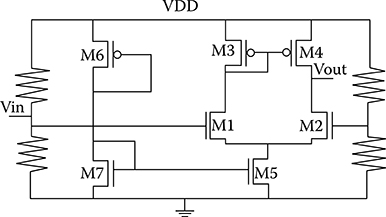
FIGURE 18.4 Amplifier topology.
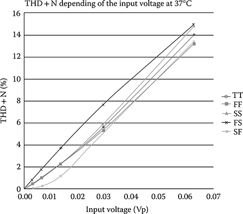
FIGURE 18.5 Amplifier THD + N Results.
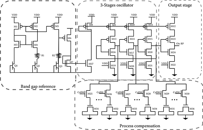
FIGURE 18.6 Oscillator topology.
The carrier frequency, permitting the RF communication, represents 45% of the system consumption with an average of 1.28 mA. Note that this circuit gives a good fit in terms of phase noise with −74 dBc/Hz at 1 MHz from the carrier.
18.6.3 Analog to Time Converter
The ramp generator is the reference element of the sampling. It is controlled by the sampling oscillator to apply a reset through the transistors M22 and M24 mounted as switches. The ramp signal has the same dynamics as the output microphone amplifier to make a comparison of these two signals.
As shown in Figure 18.7, the main part of the ramp generator is a folded cascode OTA operational amplifier. A study by Sansen [29] shows that this amplifier is a good compromise between dynamic output (1 V desired to obtain a comparison with the preamplifier) and power consumption. It should be noted that, to achieve maximum performance of this architecture, it is necessary that the current through each transistor of the differential pair (M12–M13) is equal to the mirror cascode current (M14–M17). These currents will then be added in the mirror M20–M21 to the DC bias of the output stage.
The postlayout simulations show that the dynamics of the ramp reaches a minimum of 91% of the full scale, that is, 1 V. In addition, the gain and bandwidth of the amplifier of this circuit are 33 dB and 900 kHz, respectively. Finally, this circuit, representing 21.4% of the system silicon surface, has a typical consumption of 340 μA (12% of the system consumption).
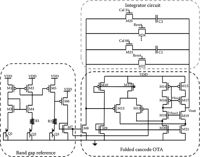
FIGURE 18.7 Integrator topology.
18.6.4 Comparator
The comparator performs the PWM. Always in the context of low power circuit, we used a two-stage comparator. Thus, for a consumption of 95 µA, this circuit has the following characteristics (postlayout simulation):
The input offset is between 250 and 320 µV.
The rise and fall time of the output signal is less than 5.4 ns (for a 10-bit signal, LSB period is 48.8 ns).
A minimum simulated bandwidth of 1.5 MHz (for a gain of 75 dB) is more than acceptable because our signal is sampled at 20 kHz.
18.6.5 Power Amplifier
This circuit has a double benefit from its implementation. First, it acts as an amplifier to ensure sufficient transmission power for communication. Then it is involved in the OOK modulation signal through the transistors M1 and M2 (Figure 18.8) functioning as complementary metal–oxide–semiconductor (CMOS) switches and supplying the amplifier as a function of the state of the PWM signal from the comparator. These electrical characteristics expressed below are derived from postlayout simulation. One decibel compression point is around −16 dBm while the input signal has an approximate value of −30 dBm and the noise figure (NF) varies between 2.4 and 2.9 dB depending on the manufacturing process.
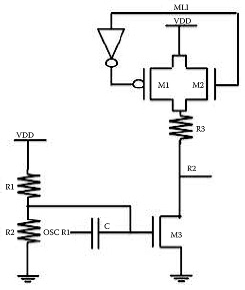
FIGURE 18.8 Power amplifier topology.
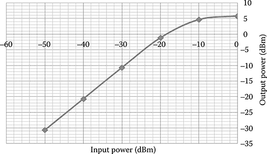
FIGURE 18.9 Power amplifier characteristics.
Figure 18.9 shows the output power as a function of input power at 37°C for a Typical (NMOS)–Typical (PMOS) (TT) process. Thus, a gain of 20 dB can be observed (at −30 dBm input) in the linear part of the power response. To improve the system consumption, the class-A power amplifier will be changed in the future by a class-C power amplifier.
18.6.6 Process Compensation
The main circuit of the calibration is a flash ADC. This architecture was chosen to have a fast processing time. Furthermore, a study by Allen and Holberg [30] shows that the silicon surface for a flash converter is smaller than a successive approximation register converter if the resolution does not exceed 5 bits.
However, two points are negative with this implementation. First, having to calibrate two oscillators and the simple ramp requires using three different ADC. This constraint greatly increases the silicon surface. To overcome this problem, we propose to implement a simple digital controller and an output memory system to perform the three calibrations with only one converter.
The second problem, solved by using the digital controller too, is the power consumption. The converter is used only during the calibration time. So, to reduce the consumption, it will be activated just during the first microsecond (4 clock cycles). After the conversion and the memorization of the three calibrations, an end of conversion signal (EOC) will turn off the power. The ADC consumption will be negligible compared with the consumption of the whole system.
For the calibration, we generate four control digital signals arriving one by one into a state machine. The first three signals enable the corresponding analog signal and the flip-flop storage to calibrate the three different components. The last signal is an EOC to control the digital controller.
The analog multiplexer retrieves the analog signal to compare within the ADC. And after, the conversion value is stored into the flip-flop. At the four clock cycles, the digital controller turns off the ADC. This architecture is illustrated in Figure 18.10.
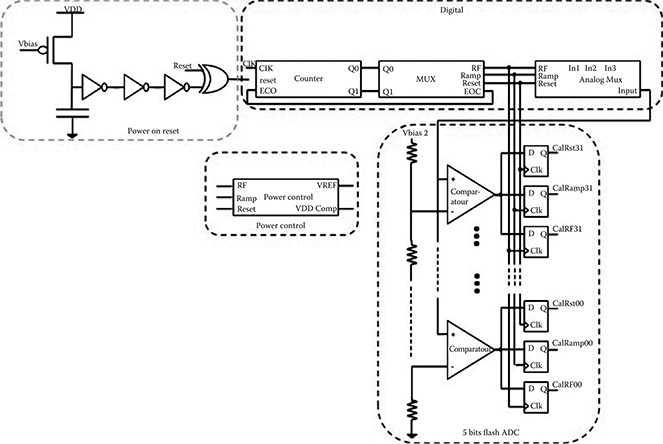
FIGURE 18.10 Low power compensation system architecture.
We will present, here, only comparison results of the dependent process block. These simulations were postlayout simulation at 37°C (typical temperature of the human body). Table 18.3 shows a comparison between the frequencies of the two oscillators with and without compensation. We can notice that, in the Slow-Fast (SF) process, the sampling frequency does not go down below 22.2 kHz due to a too important frequency shift caused by the layout (only 5 bits on the calibration converter).
18.7 Implementation and Experimental Results
This circuit has been implemented in a 130 nm CMOS technology from ST Microelectronics with an area of 1 mm2. Figure 18.11 shows the layout of the chip on the left and an element representation on the right. For test, this circuit has been encapsulated in a 3 × 3 mm2 Quad Flat No-Lead 16 package and integrated into a 6 × 2 cm2 PCB including a microphone, a battery, a 1.2 V LDO, and verification elements (Figure 18.12). The circuit consumption is approximately 3 mA.
First, the tests validate the transmitter. Figure 18.13 shows the validation of the audio amplifier, channel 1, a signal from the microphone, and channel 2, the same signal after amplification. Subsequently, the different internal analog signals were validated. To realize the PWM signal quality, the sampling frequency was increased to 40 kHz on this test. Figure 18.14 is used to realize the result. We can observe the preamplified input signal at 2.2 kHz (channel 3), the ramp conversion at 40 kHz (channel 1), and the PWM (channel 2) resulting from the comparison of the two previous signals. We can see in this picture that the analog-time conversion is not a problem in spite of a larger sampling frequency than in the specifications.
Table 18.3 Oscillators Frequencies with and without Compensation
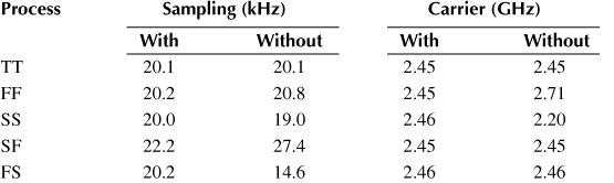
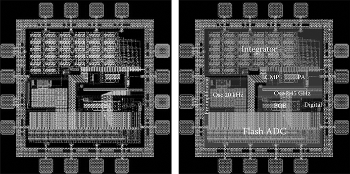
FIGURE 18.11 Transmitter layout.
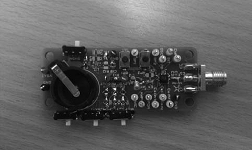
FIGURE 18.12 Transmitter test printed circuit board.
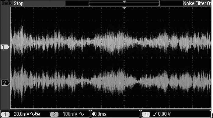
FIGURE 18.13 Microphone acquisition (channel 1) and amplifier output (channel 2).
Then, the principle of analog demodulation receiver has been validated (Figure 18.15). This measure, combining the two modules (transmitter and receiver), was made without RF communication. Thus, as shown in Figure 18.16, a 7-kHz sine was injected into the system (channel 4). Then, the comparison of this signal with the ramp sampling (channel 2), results in the PWM modulation represented in channel 1 in this figure. This signal is then injected on the input filter of the receiver to not use the RF demodulation and to highlight the final signal to be sent to the speakers (channel 3). This test highlights the proper functioning of the analog modulation produced in the transmitter and the demodulation in the receiver. It should be noted that the output signal at 7 kHz shows no distortion introduced by the electronic transceiver.
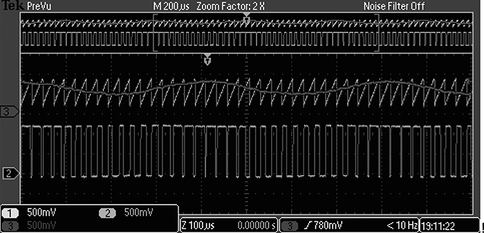
FIGURE 18.14 Internal analog signal of the transmitter.
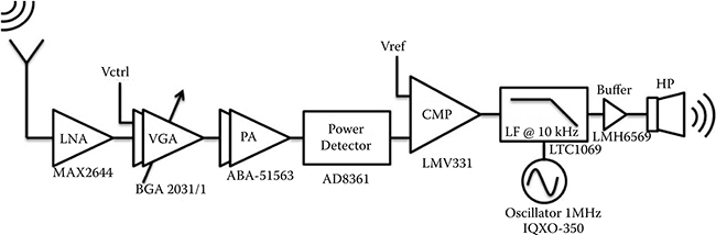
FIGURE 18.15 Receiver architecture.
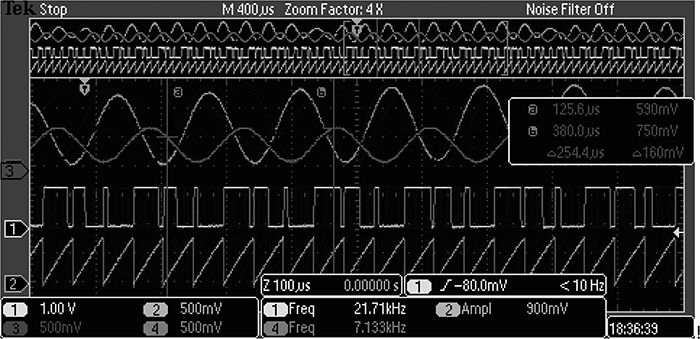
FIGURE 18.16 Analog acquisition and transmission of a 7 kHz.
Finally, the complete system has been tested, first, the RF emission whose spectrum is shown in Figure 18.17. Figures 18.18 and 18.19 illustrate the general function of the system. Figure 18.18 illustrates the acquisition of a 2-kHz sine (channel 1) and the signal returned to the speakers after the RF link (channel 2). The channel “M” curve shows the fast Fourier transform of the output signal whose amplitude is −28 dB at a frequency of 2 kHz and −75.1 dB at the first harmonic (4 kHz).
Then, we present in Figure 18.19 a realistic audio signal at the microphone input (channel 1), the amplified signal (channel 2) and the restored signal at the input of the speakers (channel 4). This acquisition is realized at 1-m RF communication with antennas presented at IEEE IWAT Conference [31]. We can observe on this oscilloscope capture the audio signal corresponding to a hissing on the microphone at different points in the system where information is purely analog. The good agreement between these curves is used to validate the chip emission and the entire demonstrator.
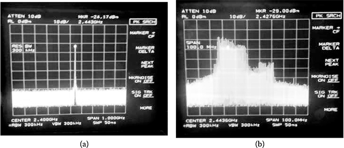
FIGURE 18.17 Transmitter spectrum: (a) without pulse width modulation and (b) with pulse width modulation.
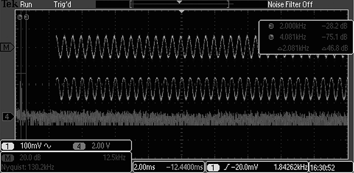
FIGURE 18.18 Top to bottom: two-kHz sine on the microphone, output signal on the speakers, and its fast Fourier transform.
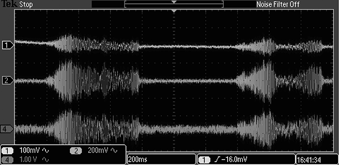
FIGURE 18.19 Top to bottom: audio signal acquisition, amplified signal, and output signal on the speakers.
References
1. J. J. Rice, B. J. May, G. A. Spirou, and E. D. Young, “Pinna-based spectral cues for sound localization in cat,” Hear Res, 58(2): 132–152, March 1992.
2. A. D. Musicant and R. A. Butler, “The influence of pinnae-based spectral cues on sound localization,” J Acoust Soc Am, 75(4): 1195–1200, April 1984.
3. R. Aibara, J. T. Welsh, S. Puria, and R. L. Goode, “Human middle-ear sound transfer function and cochlear input impedance,” Hear. Res., 152(1–2): 100–109, February 2001.
4. W. Niemeyer and G. Sesterhenn, “Calculating the hearing threshold from the stapedius reflex threshold for different sound stimuli,” Audiology, 13(5): 421–427, 1974.
5. G. Flottorp, G. Djupesland, and F. Winther, “The acoustic stapedius reflex in relation to critical bandwidth,” J. Acoust. Soc. Am., 49(2B): 457–461, August 2005.
6. E. Borg and J. E. Zakrisson, “Stapedius reflex and speech features,” J. Acoust. Soc Am., 54(2): 525–527, August 2005.
7. G. von Bekezy, “Current status of theories of hearing,” Science, 123(3201): 779–783, May 1956.
8. J. Shargorodsky, S. G. Curhan, G. C. Curhan, and R. Eavey, “Change in prevalence of hearing loss in U.S. adolescents,” JAMA, 304(7): 772–778, August 2010.
9. F. R. Lin, R. Thorpe, S. Gordon-Salant, and L. Ferrucci, “Hearing loss prevalence and risk factors among older adults in the United States,” J. Gerontol. A. Biol. Sci. Med. Sci., 66A(5): 582–590, May 2011.
10. E. B. Teunissen and W. R. Cremers, “Classification of congenital middle ear anomalies. Report on 144 ears,” Ann. Otol. Rhinol. Laryngol., 102(8) Pt 1: 606–612, August 1993.
11. C. Parahy and F. H. Linthicum, “Otosclerosis and Otospongiosis: Clinical and histological comparisons,” The Laryngoscope, 94(4): 508–512, 1984.
12. R. Dass and S. S. Makhni, “Ossification of ear ossicles: The stapes,” Arch. Otolaryngol., 84(3): 306–312, September 1966.
13. P. W. Slater, F. M. Rizer, A. G. Schuring, and W. H. Lippy, “Practical use of total and partial ossicular replacement prostheses in ossiculoplasty,” The Laryngoscope, 107(9): 1193–1198, 1997.
14. T. Shinohara, K. Gyo, T. Saiki, and N. Yanagihara, “Ossiculoplasty using hydroxyapatite prostheses: Long-term results,” Clin. Otolaryngol Allied Sci., 25(4): 287–292, 2000.
15. C. A. J. Dun, H. T. Faber, M. J. F. de Wolf, C. Cremers, and M. K. S. Hol, “An overview of different systems: The bone-anchored hearing aid,” Adv. Otorhinolaryngol, 71: 22–31, 2011.
16. P. Westerkull, “The Ponto bone-anchored hearing system,” Adv. Otorhinolaryngol, 71: 32–40, 2011.
17. D. A. Scott, M. L. Kraft, E. M. Stone, V. C. Sheffield, and R. J. H. Smith, “Connexin mutations and hearing loss,” Nature, 391(6662): 32–32, January 1998.
18. N. E. Morton, “Genetic epidemiology of hearing impairment,” Ann. NY Acad. Sci., 630(1): 16–31, 1991.
19. F. G. Zeng, “Trends in cochlear implants,” Trends Amplif., 8(1): 1–34, 2004.
20. U. Kawoos, R. V. Warty, F. A. Kralick, M. R. Tofighi, and A. Rosen, “Issues in wireless intracranial pressure monitoring at microwave frequencies,” PIERS, 3(6): 927–931, 2007.
21. Knowles Electronics, Datasheet microphone FG-6107-C34, available at http://www.knowles.com, accessed 2012.
22. ZeniPower, Datasheet pile A10, available at http://www.zenipower.com/en/products005.html?proTypeID=100009376&proTypeName=A10%20Series, accessed 2012.
23. ISM 2.4 GHz Standard, ETSI EN 300 440-1/2, v1.1.1, 2000-07.
24. O. Diop, F. Ferrero, A. Diallo, G. Jacquemod, C. Laporte, H. Ezzeddine, and C. Luxey, “Planar antennas on integrated passive device technology for biomedical applications,” IEEE iWAT Conference, Tucson, AZ, pp. 217–220, 2012.
25. F. Merli, L. Bolomey, E. Meurville, and A. K. Skrivervik, “Dual band antenna for subcutaneaous telemetry applications,” Antennas and Propagation Society International Symposium, Toronto, Canada, pp. 1–4, 2010.
26. Maxim Integrated, MAXIM IC, Datasheet Amplificateur faible bruit MAX2644, available at http://www.maxim-ic.com/datasheet/index.mvp/id/2357.
27. F. Cilek, K. Seemann, D. Brenk, J. Essel, J. Heidrinch, R. Weigel, and G. Holweg, “Ultra low power oscillator for UHF RFID transponder,” IEEE International Frequency Control Symposium, Honolulu, HI, pp. 418–421, 2008.
28. R. Chebli, X. Zhao, and M. Sawan, “A wide tuning range voltage-controlled ring oscillator dedicated to ultrasound transmitter,” IEEE International Conference of Microelectronics, Tunis, Tunisia, ICM, 2004.
29. W. M. C. Sansen, Analog Design Essentials, Springer, Dordrecht, the Netherlands, 2006.
30. P. E. Allen and D. R. Holberg, CMOS Analog Circuit Design, 2nd ed. Oxford University Press, New York, pp. 445–449, 2002.
31. O. Diop, F. Ferrero, A. Diallo, G. Jacquemod, C. Laporte, H. Ezzeddine, and C. Luxey, “Planar antennas on Integrated Passive Device technology for biomedical applications,” IEEE iWAT Conference, Tucson, AZ, pp. 217–220, 2012.