Keywords

Wind power assessment; wind energy; forecasting wind power; site selection; micrositing

3.1 Introduction

Wind is one of the prominent renewable energy resources. The percentage of wind energy–based resources for electricity generation has been steadily growing. Currently Denmark is producing over 40% of its electricity from wind-based resources [1]. There is a strong growth pattern in terms of the installed wind capacity. To cite an instance, the installed worldwide wind capacity reached 432 419 MW at the end of 2015. When compared with the figures of 2014, this represents an increase of nearly 17% (i.e., this figure was 369 695 MW at the end of 2014) [2]. The adoption rates of utilizing wind-based resources for generating wind energy, as expected, are different throughout various regions in the world. In the United States, 4% of the total electricity is obtained from wind-based resources, while the State of Iowa produces 31% of the electricity from wind-based resources [3].

To assess the wind energy feasibility at a particular site, it is imperative to conduct a successful wind resource assessment and measuring program. To embark on such a study, it is important to develop a sound quality assurance plan and framework associated with each wind potential program. The measurement, equipment, and apparatus selection that have acceptable standards, data collection, and analysis schemes are important aspects to consider.

Usually, wind potential assessment programs consist of several important steps. These can be listed as preliminary area identification, area wind resource evaluation, and micrositing (i.e., choosing the best location for wind turbines within the wind potential assessment site) [4]. Those aspects are discussed in more detail in the following sections.

The first wind resource assessment program starts with wind atlases (i.e., wind resource maps) depicting the wind potential. The data obtained from satellites is now being used extensively along with the data obtained from ground resources. To cite an instance, Solar and Wind Energy Resource Assessment (SWERA) project for the United Nations Environment Programme is one of the extensive initiatives that have been formed for this purpose [5].

During the recent decades, considerable effort has been spent on improving the accuracy and detailing level of wind atlases. To improve the accuracy, extensive network of ground measurement units must be deployed. With the inclusion of the satellite and remotely obtained data, the accuracy and resolution of the atlases should significantly improve. As such, there is an ongoing effort initiated by the International Renewable Energy Agency to combine the publicly available Geographic Information System (GIS) data to obtain a comprehensive picture of the available wind resources. For this purpose the Energy Sector Management Assistance Program (ESMAP) has allocated US$22.5 million for supporting the projects conducted over 12 different countries until 2018 [6]. However, it should be also kept in mind that there is a need for actual field work no matter how detailed and accurate the wind atlases are. The data should be validated for short-, medium-, and long-term time periods for tapping the whole potential of a wind site.

The outline of the chapter is as follows. In Section 3.2, we discuss the main principles associated with developing a successful wind assessment program. In Section 3.3, we outline the main aspects of a wind potential assessment program which involves instrumentation, data handling, preliminary analysis, and hind-sight analysis such as Measure-Correlate-Predict (i.e., MCP). In Section 3.4, the methods for obtaining the average wind power based on wind speed measurements are described. In Section 3.5, we discuss the aspects associated with the wind assessment such as the scale of analysis (i.e., microscale, mesoscale, and macroscale), the analytical models and software that might be utilized for the siting purposes, (e.g., Wind Atlas Analysis and Application Program (WAsP), Computational Fluid Dynamics (CFD)-based approaches, and the spatial exploration models. In Section 3.6, we provide additional considerations associated with wind resource assessment such as extreme wind speed analysis, rugged terrain analysis, wake of turbines, uncertainty analysis, and estimation of losses associated with electricity production. In Section 3.7, we summarize the analytical approaches associated with the forecasting of wind speed and wind power. In Section 3.8, we provide overall conclusive remarks.

3.2 Principles for Successful Development for a Wind Assessment Program

A successful wind assessment program includes: site identification, preliminary resource assessment, and micrositing according to New York State Energy Research and Development Authority [8], with wind atlases serving as a valuable tool for preliminary analysis. Apart from using wind atlases, there are additional steps that should be performed. These are identified as: (1) instantaneous wind speed measurement to estimate the wind potential; (2) interviewing stakeholders regarding the environmental impact of the wind turbines; (3) studying the meteorological information regarding the wind speed and wind direction; (4) availability of land; and (5) terrain features, i.e., surveying the obstructions that might impede the wind flow [7].

In general, a preliminary resource assessment includes defined measurement plans where the key decisions on the tower placement, height, and instrumentation are given. Besides those decisions, the determination of whether adequate wind resources exist within the specified area, a comparison of different areas for distinguishing relative development potential, obtaining representative data for the estimation of economic viability and performance of wind turbines, and the screening of the potential of wind turbine installation sites are also important considerations [4].

Regarding micrositing, the main aspects of decision-making involve conducting additional measurements for validating the data, conducting the necessary adjustments for the wind shear and the long-term wind climate, numerical flow modeling, and the corresponding uncertainty estimation. Moreover, in the micrositing phase, small-scale variability of the wind resource over the terrain of interest is quantified to position one or more wind turbines to maximize overall energy output [8].

Wind atlases are the starting point for a preliminary site selection. However, it should be kept in mind that these maps give only a rough estimate and might differ from the actual wind speeds by ±10%–15%. Since wind power is a function of the cube of the wind speed, the deviation between actual and estimated wind output could be further compounded; this might lead to the differences of up to ±20% [9].

Usually, the classification of wind sites with respect to wind potential is on a five-scale rating. According to this classification, class-5 is considered as extremely suitable for a wind farm, whereas class-1 is deemed as unfeasible. In that regard, Bennui et al. [10] use GIS and employ a multiple decision criteria–based method to classify wind sites. The decision criteria are: wind speed information, elevation, slope, highways and railways, built-up area, forest zone, and scenic area.

Researchers have developed comprehensive methods for assessing wind potential. To cite an instance, Lawan et al. [11] conduct a structured analysis and review the steps for conducting the wind resource assessment program for Malaysia. They also discuss the prospects and challenges of using wind energy both in the developing and developed countries. It is believed that the developing countries especially in Asia have untapped potential for wind energy and suggested that the government and private entities should work together, especially for harvesting wind energy in remote and rural areas. It is also pointed out that wind speed distribution, energy potential modeling, determining cut-in, cut-out and rated wind turbine velocities, wind speed profiling, and proper software selection are important aspects once the wind potential is properly assessed.

In a similar fashion, there are some analytical methods used for comparing wind potentials at different sites. Corbett et al. [12] develop a methodology based on the CFD approach for comparing 13 wind farm sites involving 74 mast pairs. The CFD-based approach should be fine-tuned with respect to the flow characteristics of the wind, using care, expertise, and engineering judgment especially for complex terrain conditions. Additionally, wind assessment programs could play a pivotal role in shaping the decisions. For instance, Wang et al. [13] emphasize the importance of holistic approaches that would necessitate the integration challenges associated with the Chinese wind energy policies. To obtain full potential of wind-based resources, it is vital to determine the predictability with successful forecasting models, and improve energy markets with the objectives of long-term development and pricing reforms. To enhance predictability and creating effective markets, research and development on wind resource assessment programs are of paramount interest and these activities should be conducted in a transparent manner. The steps that should be conducted for realizing a successful wind energy system is given in Fig. 3.1.

3.3 Main Aspects of a Wind Assessment Program

One of the most important parameters in determining the electric power obtained from the wind-based resources is wind speed. The general equation relating wind power to swept area, wind speed, and density of air is [7]:

$P_w=\frac{1}{2}\rho A{v}^3$ (3.1)

(3.1)

where P_w is the wind power, ρ is the density of the air, and v is the wind speed. This represents the total energy obtained from the wind flow. In terms of generating electric energy, only a certain proportion of the kinetic energy of the wind can be converted. This relation can be expressed as,

$P_e={\eta }_e{\eta }_m{C}_p{P}_w$ (3.2)

(3.2)

where P_e is the amount of electric power generated, η_e is the electric conversion efficiency of the wind turbine, η_m is the mechanical efficiency, and C_p is the power coefficient. The upper limit for the power coefficient (i.e., the proportion of the amount that can be extracted from the kinetic energy of the wind) is 59.3% regardless of the geometry of the wind turbine. Usually the power coefficient of the modern wind turbines is between 45% and 50% [15]. Fig. 3.2 is a typical power curve of a wind turbine that shows the relation between the generated wind power and the wind speed.

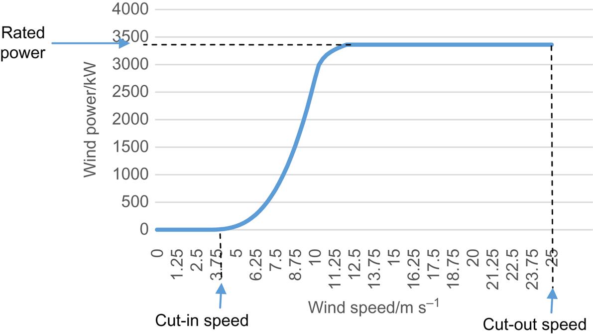
As illustrated in Fig. 3.2, at low wind speeds, there is not enough torque applied by the wind to generate electricity. The minimum wind speed at which electricity can be generated is called the cut-in speed, namely, the speed at which the rotor of the wind turbine begins turning. As described in Eqs. (3.1) and (3.2), the generated wind power increases with the cube power of the wind speed, up to a certain value which is called rated power. The rated output is usually obtained at the maximum speed that the rotor is allowed to turn. Usually, the wind turbine manufacturers place an upper limit on the speed that the blades are allowed to turn to increase the longevity of the blades by preventing and minimizing bird impacts, rain, erosion, etc. [16]. Typically, the tip of the blade of the rotor turns at a maximum speed of 120 m s⁻¹. Turning the blades faster could lead to problems. Beyond a certain speed, in order to prevent structural damages, the rotor is brought to a standstill by a brake. This particular wind speed is called the cut-out wind speed.

To determine the potential of a wind-based resource to the fullest extent, identification and survey of the site are the most vital concern. For this purpose, proper instrumentation plays a crucial role. Wind power maps give only a crude information regarding the specific information sites. To characterize the wind-related properties, and collect associated data, a sound data acquisition program with the following aspects should be taken into consideration [8]:

Some consider placing remote sensing equipment for collecting the wind-related data. In a study conducted by Rodrigo et al. [17], the procedures for the testing and evaluation of the remote sensing equipment for the wind-related attributes were investigated. For this purpose, two terrains with different topologies (i.e., a flat and a complex terrain) are considered. An intercomparison between sound- and light-based equipment (i.e., SODAR—Sound Detection and Ranging system and LIDAR—Light Detection and Ranging system) that can remotely sense the wind is made. The researchers use a single-point regression, ensemble-averaged profile analysis, and a performance matrix in the evaluation steps and discuss the principles associated with the remote sensing equipment for a wide variety of terrain conditions. The analysis is helpful for extending the scope of the wind energy potential assessment campaigns and measuring the corresponding wind attributes at certain heights without the need for installing anemometers at specified distances. It is concluded that although the remote sensing technologies using the sound and light wave technologies show improvement, defining standards for testing and calibration is difficult for the complex terrain applications. It is also indicated that a multitude of prototype designs in terms of the uncertainty of the measurements with respect to various terrain conditions should be evaluated for remote sensing equipment in order to develop standards for generating bankable data.

For the wind turbines located offshore, other approaches are of interest. To cite an instance, Nicholls-Lee [18] discusses the possibility of instrumentation platforms that have the mobility deployed for assessing of wind potential offshore. The feasibility of lightweight, floating platform for a repositionable meteorological measurement station is evaluated. Contrary to the traditional anemometers, LIDAR is adopted for capturing the wind speed and direction at the specified heights. Such a platform could be a viable alternative to deploying costly masts to capture the offshore wind potential. Other researchers discuss the potential for utilizing the data captured by satellites for conducting wind resource assessment [19,20].

Aside from the wind speed, one of the most important wind attributes is the ambient air temperature. The air temperature determines the air density. As indicated in Eq. (3.3), wind power increases with the air density. The relation between the air temperature and the air density for humid air can be approximated using the ideal gas formula;

${\rho }_{\mathrm{humid\; air}}=\frac{p_d}{R_{d}T}+\frac{p_v}{R_{v}T}$ (3.3)

(3.3)

where ρ_{humid air} is the density of humid air (in kg m⁻³), p_d is the partial pressure of the dry air (in Pascal), T is the temperature (in Kelvin), R_d is the specific gas constant for dry air (i.e., 287.058 J (kg K)⁻¹), p_v is the partial pressure of the water vapor (in Pascal), and R_v is the specific gas constant for water vapor (i.e., 461.495 J (kg K)⁻¹). The temperature readings should be conducted at several meters above the ground to minimize the effects of surface heating [7].

Another consideration is the determination of the distance between the measurement point and the potential location of the wind turbine. It should be kept in mind that as the terrain becomes more complex due to the variability associated with the local wind characteristics, the maximum distance between the point of measurement and the potential location should decrease. As a rule of thumb, that distance should be 5–8 km for a relatively simple terrain, and 1–3 km for the regions where complex terrain conditions are present (e.g., steep geometrically complex ridgelines, coastal sites with varying distance from the shore or heavily forested areas) [8]. This necessitates the placement of a larger number of measurement towers for wind farms as compared to stand-alone turbines. Intuitively, the number of towers should be increased to analyze the perturbation of the more complex terrain on the wind flow. In that regard, the tower placement should be representative of the turbine locations. Nevertheless, in order to obtain a comprehensive picture and analyze the wind flow over an area more accurately, some towers should also be placed at the coordinates where less than ideal conditions exist [21].

For deciding on the final location of turbines, a preliminary analysis needs to be conducted using software (e.g., WindPRO) based on the wind resource maps and terrain-based constraints. The siting of wind turbines at a location involves grouping turbines into clusters based on distance. For relatively flat terrains, the rule of thumb is to place 10–12 turbines in one cluster, and for more complex terrains, place 5–7 wind turbines in one cluster. After forming the cluster, the median wind speed within the cluster is calculated based on the wind resource map, and the locations at which the median speed is observed are selected for the potential location for the measurement points and hence the construction of towers. Usually, two or three candidate locations are selected for a tower. Then, by visual examination, the final locations of those towers (one for each cluster) are selected in such a way that those towers are sufficiently spread out [22].

Furthermore, consideration should be given to the extrapolation of data obtained from different wind sites. The following simple equation might be used for this purpose [8]:

$v_2=v_1{\left(\frac{h_2}{h_1}\right)}^{\alpha }$ (3.4)

(3.4)

where v₁ is the known speed at measurement height h₁, v₂ denotes the wind speed at the height h₂ where the wind speed is extrapolated, and α is the wind shear exponent. There are various factors that affect the wind shear exponent, including vegetation cover, terrain, general climate, and even the time of the day. In the literature, α values ranging between 0 and 0.4 are reported [8].

Not only the new measurement facilities, but also the existing measurement units might be used for wind resource assessment. For this purpose, existing towers, airport measurement units, and spatial extrapolation models might be used. Waewsak et al. use 120 m wind tower at the shoreline to analyze the monthly mean wind speeds and dominant wind directions. Using this data, they obtain a 20 m resolution microscale map, and estimate the annual energy productions, wake effects, and theoretical capacity factors [23]. In a similar fashion, Kim and Kim [24] use the AMOS (Aerodrome Meteorological Observation System) wind data measured at Yeosu Airport to develop a wind resource map. Based on this map and by employing three cases with different designs for the wind turbine, a comparative economic analysis is conducted.

Generally, MCP can be defined as the collection of methods that are used for the estimation of long-term wind resources based on short-term data. The idea is about using the short-term campaign and correlating it with an overlapping but climatologically representative time series (i.e., 5 years, preferably 10 years) [25]. The larger the wind project becomes (in terms of installed capacity, power rating, or similar performance measures), the more important the accurate prediction of the wind resources. For smaller projects (i.e., for wind farms with less than 100 MW output), the length of time for recording measurements varies between 4 and 6 weeks [8]. However, for larger projects long-term measurements might be needed for capturing the differences due to the change of seasons, or factors associated with a complex terrain. The methods that have been used to extrapolate data for long-term performance began in the 1940s for single stations, and gradually evolved into more complex methods. Those early methods usually use linear, nonlinear, and probabilistic transfer functions and could be applied to a time series data as well as to frequency distributions of associated wind speeds [26].

3.4 Estimating Wind Power Based on Wind Speed Measurements

After the data acquisition and validation phase, the next step is to analyze the data for estimating the wind energy that would be produced over a certain period. As previously indicated, the wind speed varies over time and statistical distributions might be employed for this case. Weibull distributions are usually employed for modeling wind speed distributions [27]. Based on this assumption, the following model can be used to estimate the wind power output. Following Eq. (4.5), the average wind power can be calculated as [28]:

$P_{\mathit{ave}}={\zeta P}_E$ (3.5)

(3.5)

where $P_{\mathit{ave}}$ is the average wind factor, $\zeta$ is the capacity factor, and P_E is the electricity power generated. To find the $\zeta$ value, the following integral should be evaluated;

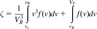$\zeta =\frac{1}{V_R^3}\underset{v_c}{\overset{v_R}{\int }}{v}^{3}f\left(v\right)\mathit{dv}+\underset{v_R}{\overset{V_F}{\int }}f\left(v\right)\mathit{dv}$ (3.6)

(3.6)

where $V_R$ is the wind speed at which the rated power is reached, v_c is the cut-in speed, $V_F$ is the cut-out speed, and f(v) is the probability density function of the wind speed. Assuming that the Weibull distribution, which is one of the most widely used distribution for characterizing wind speed, is used, $\zeta$ can be calculated as:

$\zeta ={\left(\frac{v_c}{v_R}\right)}^3{e}^{{{-(v}_c/c)}^k}+3\frac{\mathrm{\Gamma }(\frac{3}{k})}{k}{\left(\frac{v_R}{c}\right)}^3\left[\gamma \left({\left(\frac{v_R}{c}\right)}^k,\frac{3}{k}\right)-\gamma \left({\left(\frac{v_c}{c}\right)}^k,\frac{3}{k}\right)\right]-e^{{(v_f/c)}^k}$ (3.7)

(3.7)

where $\left(v_R/c\right)$ is the normalized rated speed, $\mathrm{\Gamma }$ is the gamma function, $\gamma$ is the incomplete gamma function, c is the Weibull scale parameter, and k is the shape parameter.

The Weibull scale parameter can be estimated from the following equation:

$k={\left(\frac{\sigma }{\overline{x}}\right)}^{-1.086}$ (3.8)

(3.8)

$\frac{c}{\overline{x}}={\left(0.568+\frac{0.433}{k}\right)}^{\frac{-1}{k}}$ (3.9)

(3.9)

where σ is the standard deviation of the wind speed and $\overline{x}$ is the average wind speed.

Various approaches have been used for determining the underlying distribution governing the wind speed equation. Zhou et al. [29] have compared various distributions for modeling the wind speed distribution, and conclude that the maximum entropy–based functions proved to be a versatile tool. The authors conduct a comprehensive study on five North Dakota Sites and indicate that no distribution outperforms any others but Rayleigh-based distributions in general are inferior when compared to other distributions (e.g., maximum entropy based, Weibull, Rayleigh, gamma, lognormal, and inverse Gaussian). Some researchers have used the bivariate distribution for modeling and characterizing wind attributes (i.e., direction and speed) simultaneously. Erdem et al. [30] provide a comparison for modeling the wind speed and direction using three different approaches (namely, angular-linear, Farlie–Gumbel–Morgenstern (FGM) and anisotropic lognormal approaches), in terms of the root mean square error and R² values. The FGM approach provides compatible results, while the anisotropic normal distribution lags behind. Fractional distributions can also be used for modeling the wind speed distributions, e.g., the fractional Weibull distributions [31]. Some researchers develop nontraditional methods for characterizing the wind speed distributions over a long period of time. Li and Shi [32] combine an averaging Bayesian model and Markov Chain Monte Carlo sampling methods, and conclude that the combined approach provided comparative reliability and robustness in describing the long-term wind speed distributions for the selected wind sites.

3.5 Wind Resource Estimation Project: Scope and Methods

In terms of the scope, wind resource assessment can be conducted at different levels (i.e., microscale, mesoscale, and macroscale). As the name implies, microscale wind resource assessment campaigns usually entails assessing the wind power for a smaller region such as the local/site coverage; mesoscale entails the national coverage; and macroscale usually focuses on estimating the wind potential on a global scale. The resolution of the wind power assessment program differs widely with respect to scale. In general, microscale entails a resolution of between 10 and 100 m; mesoscale entails the resolution of approximately 5 km; and macroscale incorporates a resolution of approximately 50–200 km [33].

The estimates for global wind power vary depending on the assumptions and associated constraints. Most researchers evaluate the potential of both onshore and offshore winds. The estimate for total wind potential varies considerably. Lu et al. [34] predict the global wind energy potential to be 840 000 TW h per year based on the Goddard Earth Observing System Data Assimilation System (GEOS-5 DAS) dataset. This dataset uses a weather/climate model incorporating inputs from a wide variety of observational sources (surface and sound measurements) and a suite of measurements and observations from a combination of airborne vehicles (i.e., aircraft, balloons, ships, and drones), sea units (ships and buoys), and satellites. This creates fairly accurate high-resolution wind potential maps. The authors indicate that 36% of the capacity factor is the breakeven point for satisfying the world demand for electricity power if those wind turbines are only located onshore. On the other hand, Hoogwijk and Graus [35] by employing a more constrained model, estimate that the global capacity for wind-based resources for generating electricity is 110 000 TW h per year. The authors indicate that the theoretical potential involves natural and climatic factors, while geographical potential involves examining land use and land cover limitations. It is also indicated that market potential involves demand for energy, competing technologies, and examining corresponding policies and measures.

As previously described, various models are employed for describing wind flow. These models, usually used for micrositing decisions, can be divided into four categories: conceptual, experimental, statistical, and numerical [8]. As the name implies, conceptual models refer to the basic concepts and discuss how wind flow is affected by the terrain. Some researchers employ the conceptual models to quantify the effects of offshore and coastal wind turbines on the ecology. To cite an instance, Wilson et al. [36] use those models to evaluate the impact of offshore wind turbines and the associated infrastructure (e.g., substations and subsea cables, etc.) on the sea life.

Experimental models usually involve creating physical models of the terrain, and experimentally studying the actual flow. Experimental models are traditionally employed for testing wind turbine designs or validating analytical wind flow models [37,38]. Usually those designs necessitate the use of wind tunnels or related equipment. Recently, other means have been developed. For example, Conan et al. [39] use sand erosion model to detect and evaluate high wind speed areas for wind power estimation. This model is low cost, easy to build, and repeatable, and it can be used to estimate the wind characteristics such as the amplification factor and the fractional speed-up ratio.

Statistical models aim at finding the relation between various terrain characteristics (e.g., surface roughness, elevation, and slope exposure) and the wind power [8]. Shahab et al. [40] use parametric and nonparametric statistical approaches for determining the requirements associated with an energy storage system for providing the baseload for wind farms. Forest et al. [41] use the multiple kernel learning regression for assessing the wind performance over a complex terrain. Rather than the topographic indexes to obtain the regression equation, their method is based on the support vector regression method. One advantage of the approach is that the algorithm, based on the inclusion of additional data in a nonparametric fashion, actually learns.

Numerical models can be divided into four major groups. The first group is the mass-consistent models, which are formed by the group of equations based on the principle of mass conservation. Those models were developed in 1970s and 1980s and have been used with success as approximation techniques even for the complex terrain. The success is due to their simplicity and the applicability of the physical principles governing the equations [42]. The second generation of the models that are collectively known as Jackson–Hunt based approach incorporates the conservation of momentum as well as the conservation of mass by employing Navier–Stokes type of the equations [43]. Over the years, the basic theoretical construction has been developed which has led to some widely used software packages. Among them, WAsP is a popular choice for the micrositing decisions for wind turbines [44]. The MS3DJH/3R models are used in conjunction with the mass-consistent models to study boundary layer flow over analytical two-dimensional hills with varying slope [45]. Raptor Nonlinear (Raptor NL) software is used for modeling the wind flow over the steep terrain [46].

Among the Jackson–Hunt based approach, the WAsP software has been enjoying popularity especially in Europe. It was first developed by the Technical University of Denmark in 1987 and has been further enhanced over time to incorporate different models for the projection of horizontal and vertical extrapolation of data for application over different types of terrain [47]. Various modules for WAsP have also been developed, such as the functionality to estimate the effects of surface roughness changes and obstacles [8,48].

Recently, the third group of numerical models (i.e., CFD-based approaches) is also gaining popularity thanks to increasing computing power. These approaches are usually aimed at developing a steady-state independent solution for wind and turbulence fields, which can be used for wind power assessment for complex terrains [49]. CFD models make use of the equations based on Reynolds-averaged Navier–Stokes for motion [50]. The CFD-based models can also be used for regions where thermal instability exist [22]. CFD-based approaches on the real-life problems have a mixed success. While they have been verified in the experimental setting with 2D and 3D flow with the steep hills using wind tunnels researchers report mixed results for wind power estimation for real-life cases [8,51–53].

The fourth group of numerical methods incorporates the mesoscale numerical weather prediction (MNWP) models. Those models are usually employed for weather forecasting, and can also incorporate energy and time. Such models can be used for modeling various atmospheric-related phenomena such as thermally driven mesoscale circulations, atmospheric stability, and buoyancy. Other wind-related characteristics such as pressure, humidity, and temperature can also be modeled. One of the shortcomings is that the computational resource requirements for these models are prohibitively large [14]. A general flowchart for the MNWP model is presented in Fig. 3.3.

Meanwhile, researchers have explored the feasibility of hybrid approaches. There are some applications which combine the MNWP models with the Jackson–Hunt based models or the mass-consistent models such as the AWS Truepower’s MesoMap, Risoe National Laboratory’s Karlsruhe Atmospheric Mesoscale Model-Wind Atlas Analysis and Application Program (KAMM-WAsP), and Environment Canada’s AnemoScope system [55–57].

In addition, spatial extrapolation models can be used for extrapolating the wind data obtained from one wind location to assess the potential at another wind site. Techniques based on statistics or artificial intelligence have been used for this purpose. To cite an instance, Garcia-Rojo [58] employs a procedure based on the calculation of the joint probability distribution of the wind at a local station and a meteorological mast, and compares it with the estimation of a MCP model. Some researchers employ the spatial extrapolation models for predicting the wind power in a vertical sense in such a way that the data obtained from a certain height is extrapolated to obtain an estimate for a different height. As an example, Durišić and Mikulović [59] use wind data obtained at three different locations to form a synthetic model using the method of least squares [59]. The proposed approach can also be used as a tool to refine the input for the WAsP model.

3.6 Further Considerations for Wind Speed Assessment

Wind turbines are designed to shut off to prevent damage beyond a threshold wind speed. In analyzing extreme winds, An and Pandey [60] compare four different approaches (i.e., Standard Gumbel, Modified Gumbel, Peaks-Over-Threshold (POT), and Method of Independent Storms (MIS)), and conclude that the MIS produced more reliable results as compared to other type of the methods, especially the POT method.

Terrain characteristics are also worth considering. Wind assessment becomes more difficult with increasing terrain complexity; traditional WAsP software works better for the flatter terrains. A ruggedness index can be analogously defined as the percentage of the terrain that has a slope greater than the threshold value. By calculating the index, it would be possible to develop correction procedures for the estimates obtained from the WAsP model for more complex terrains [61].

Various sources of uncertainties exist that might impede accurate assessment of wind potential at a particular site. These uncertainties can be classified as:

For a project with a life span of 10 years, the total compounded effect of uncertainties from different sources might vary between 4.1% and 7.5% [8].

The estimation of losses affects the wind potential assessment. As a rule of thumb, for the losses associated with a small wind turbine, the theoretical output must be reduced for accommodating real-world operating conditions. This deratement factor might reach up to 15%–30%. Usually, the following factors are cited as the sources for losses [62]:

The wake of the turbines is another factor. It is suggested in the literature that in order to reduce wake losses at wind farms, turbines should be spaced between 5 and 9 rotor diameters in the prevailing wind direction, and between 3 and 5 rotor diameters in the direction perpendicular to the prevailing wind [60].

3.7 Wind Speed and Power Forecasting

Since wind is an intermittent energy source, predicting a reliable supply of wind power is a challenging task that should be addressed accordingly. Accurate forecasting reduces the uncertainty and streamlines the planning activities associated with the grid. To forecast wind speed and power, numerous methods have been proposed in the literature. Depending on the time horizon associated with the forecasting period, wind forecasting can be divided into four distinct categories [65]:

There are various methods that can be employed in terms of forecasting wind speed. Fig. 3.4 provides an overview on the general classification in the literature. Persistence-based models assume the previous period value as the forecast for a future period. This method works well especially for very short-term and short-term forecasting [66]. Meanwhile, it is usually used for benchmarking purposes to test the forecasting quality of other methods.

Numerical weather prediction–based methods are usually used for forecasting the local weather and air related attributes. Various software packages for numerical weather prediction (NWP) methods have been developed, which include the High Resolution Local Area Model (HIRLAM), the hydrostatic ETA model (i.e., a hydrostatic model that employs the eta vertical coordinate), Aire Limitée Adaptation dynamique Développement International (ALADIN) model [68–70]. One striking difference between the NWP model and the other models is that various wind attributes other than wind speed can be forecasted (e.g., pressure, density, direction, temperature, and humidity) with the NWP model. However, the forecasts obtained by the NWP models depend heavily on the initial conditions; therefore providing an ensemble forecast increases the reliability of prediction. Unfortunately, the use of NWP-based methods does require a large amount of computing power, and even with the right set of the inputs, due to the chaotic behavior, forecasting the wind attributes beyond a couple of weeks ahead is usually not possible. Generally, this model performs well for the long term, but short-term predictions are inferior compared to other methods. Moreover, the NWP models, due to the high cost of collecting the input set and the high computing costs, are only used once or twice daily [65]. Since the NWP method serves as a platform for forecasting the future weather state, the output might be further processed to obtain finer estimates with respect to the wind attributes. In that regard, Cassola and Burlando [71] apply the Kalman filtering method for improving the wind speed and wind power forecasts for the very short term. Some researchers also use neural networks for postprocessing model output forecasts obtained from the NWP models [72]. In a similar sense, the output of the NWP models might be further postprocessed for identifying certain deviating patterns. For instance, Bossavy et al. [73] use the derivative filtering approach for edge detection to characterize ramp events when the power production of the wind turbine significantly deviates from the usual electricity generation pattern.

Statistical and learning–based approaches incorporate various methods from statistics and artificial intelligence. Statistical-based approaches usually incorporate techniques applied on a time series data such as Auto Regressive Integrated Moving Average (ARIMA) based methods. There are various implementations of ARIMA-based models in the literature, such as fractional ARIMA-based models and joint Auto Regressive Moving Average (i.e., ARMA) models for predicting wind attributes simultaneously [74,75]. ARMA-based models are based on the previous period’s wind speeds/power and past error terms. In general, the ARMA-based model can be expressed as [76];

$y_t=\delta +\sum _{i=1}^p{\phi }_i{y}_{t-i}+\sum _{j=1}^q{\varphi }_j{e}_{t-j}+e_t$ (3.10)

(3.10)

where $\delta$ is the constant term associated with the stochastic process of the ARMA model, ${\phi }_i$ is the ith autoregressive coefficient, ${\varphi }_j$ is the coefficient of jth moving average, $e_t$ is the error term at time period t, and $y_t$ represents the value of wind speed observed or forecasted at time period t.

In addition to the traditional static ARMA models, researchers have developed dynamic versions for capturing inherent nonstationary wind speeds. In that regard, Huang and Chalabi [77] use the smoothed integrated random walk processes to model the coefficients of model parameters. Recently, there is a growing interest in combining the traditional ARMA-based models with other approaches. In that vein, Liu et al. [78] develop two approaches where the ARMA model is linked with artificial neural network (ANN) and Kalman filter based methods, and Shi et al. [79] combine ARMA with ANN and support vector machines (SVMs) for the same purpose. It is concluded that those models perform well for the nonstationary wind speed prediction in wind power systems. The statistical-based methods are not only limited to the ARMA-based models. For instance, Liu et al. [80] adopt the Modified Taylor Kriging model and compare the forecast quality to ARMA-based approaches.

Researchers have also explored the possibility of implementing Auto-Regressive Conditional Heteroskedasticity (ARCH) and Generalized Auto-Regressive Conditional Heteroskedasticity (GARCH) based models for modeling the variability of wind speed. Those variance equations can be incorporated in the mean regression equation and (-M) counterparts can be created in this fashion. Liu et al. compare 10 different ARMA-GARCH(-M) based approaches for modeling the volatility and conclude that no model outperforms the other, and indicate that as the height increases, the power of the model decreases [81]. Those studies are important for providing the interval forecast and calculating the operation probability of the wind turbines and conditional expected wind output [82,83].

On the other hand, ANN is a technique that has been used to map the random input vector(s) to outputs without prior assumptions of a fixed relationship. The neural network can learn based on the existing data, discover the hidden patterns, and use the past data to predict future ones. Successful implementations of ANNs for wind speed forecasting exist in the literature [84,85]. Li and Shi [86] compared three different ANNs, namely adaptive linear element (ADALINE), feed-forward back-propagation (FFBP) and radial basis function (RBF) for 1 hour ahead of wind speed predictions and came to the conclusion that no model outperformed any other, and that wind sites should be evaluated in terms of the performance of different ANNs on a case-by-case approach. Bilgili et al., using a logistic sigmoid transfer function, a linear transfer function as an activation function, and resilient propagation as a learning approach, developed a model for forecasting the wind speed based on the data obtained from neighboring locations [87]. Kani and Ardehali combined ANNs and the Markov chain models to develop a combined approach for very short-term forecasting of wind speed. Markov Chain based approach is employed for capturing long-term trends [88]. Fadare used 200 year data obtained from 28 ground stations and develop a three-layered, feed-forward, back-propagation network with different configurations to forecast the wind speed in Nigeria [89]. There are also other artificial intelligence methods developed for wind speed prediction purpose such as spatial correlation–based approaches, fuzzy logic–based approaches, wavelet transforms–based approaches, entropy-based training methods [90–92], and SVM approaches [93].

Ensemble forecasting usually involves a large set of runs to predict the wind speed. Those ensemble forecasts are used for examining the future forecasts and the similarities between those outcomes are examined to obtain an insight on the reliability of forecast. As previously indicated, these models are especially useful with NWP-based models [94]. Associated with ensemble forecasting, hybrid methods are also gaining popularity. Usually hybrid methods fall into two categories. These categories can be expressed as follows [85]:

Weighting based algorithms involve the determination of the relative effectiveness of each model and assigning them a value indicating the special importance in the combined models [95]. Han and Liu [96] used the maximum entropy principle to obtain weight coefficients for six individual models (persistent, ARIMA, and four ANN-based models) for different prediction horizon times (i.e., between 1 and 6 hours). Recently reported research involved the combination of different regression algorithms by means of a so-called Multiple Architecture System (MAS). Bouzgou and Benoudjit [97] implemented the MAS to combine different regression models to forecast wind speed. Li et al. [98] developed a two-stage approach where the outputs of the forecasts from different neural networks were combined using Bayesian adaptive combination, and concluded that applying Bayesian combination on the top of the individual forecasts can significantly improved the accuracy as compared to forecasts obtained from stand-alone ANNs.

Combined approaches using the preprocessing techniques, involve decomposing the nonlinear wind speed data to stationary and regular subseries and applying filtering techniques for filtering out redundant parts [85]. Wavelet transformation–based methods are gaining popularity with these combined techniques. Lei and Ran combined a wavelet transformation with the ARMA model and indicate that the particular combined approach performs better as compared to the stand-alone ARMA-based approaches [99]. Also, it Zhang et al. combined a wavelet transformation with an ANN to obtain satisfactory results [100].

On the other hand, other approaches have taken a selection of explanatory variables and determined model parameters [85]. For example, Xingpei et al. [101] used a back-propagation neural network, where the initial weights and bias are optimized by employing genetic algorithms. It is indicated that the proposed approach performs better than only using ANNs. In a similar manner, other researchers have experimented with a simulated annealing based approach for finding the parameters of the SVMs [102].

Related research is also conducted based on the postprocessing of the error terms to identify the patterns of systematic underestimation and overestimation. As an example, Louka et al. [103] applied the Kalman filtering method to reduce the error terms for two NWP models namely SKIRON which is named after the wind which blew from the Scironian rocks in Kineta, Greece and Regional Atmospheric Modeling System (RAMS) model. Wang et al. [104] adopted the ARMA models to provide a fit for the wind speed data where the error terms were modeled using the simulated GARCH(1,1)-based approach.

3.8 Conclusions

In this chapter, we discussed various aspects of wind power assessment and forecasting. The principles of developing a successful wind assessment programs are outlined. Various models that might be used for the micrositing decisions (i.e., mass-consistent based methods, Jackson–Hunt based models, methods based on CFD, spatial correlation–based methods) are discussed. Also, the important aspects of wind resource assessment analysis such as the spacing between wind turbines, uncertainty analysis, and loss estimation are discussed. In Section 3.7, we provide the classification on the types of methods used for the wind speed and wind power forecasting with the objective of reducing the uncertainty in electricity generated from wind-based resources.

It is worth mentioning that a successful wind power assessment program entails the implementation of many tasks such as preliminary wind analysis, selection of wind sites, micrositing, and accurate capture of existing wind flow profiles. Not only is the assessment of the wind power important, but also the accurate forecasts of wind speed and wind power are important considerations for tapping the full potential of wind-based resources.