
Aerodynamics and Design of Horizontal-Axis Wind Turbines
Martin O.L. Hansen, Technical University of Denmark, Lyngby, Denmark
Abstract
This chapter tries first to explain how the aerodynamic forces on a wind turbine rotor extract power from the wind by slowing down the wind speed and at the same time produce the torque needed to drive an electrical generator. Next is shown in detail how these forces and the extracted power can be computed for a given blade geometry, wind speed, and angular velocity. Such an analysis tool is needed when designing efficient blades by coupling it with a formal optimization algorithm aiming at making a rotor that in its design lifetime will capture as much energy from the wind as possible and thus help to produce electrical energy as cheaply as possible. Also the challenges of a wind turbine to overcome the tear and wear from the fluctuating loads experienced by the construction when erected in a natural inflow are addressed and are an important part in the design process.
Keywords
Wind turbine aerodynamics; wind turbine blade design thrust and power curves
9.1 Introduction
A wind turbine is a device that transforms the kinetic energy in the wind into electricity, and the overall object is to make a machine that will survive all the expected loads in the design lifetime of typically 20 years and to produce electrical energy as cheap as possible, i.e., more formally to minimize the Levelized Cost of Energy (LCoE) and usually expressed in terms of dollars per kilowatt hour. To do this one must know something about the environmental input to the wind turbine as related to wind speed distribution, atmospheric turbulence and for an offshore wind turbine also a description of the sea state. Standards/norms, such as the International Electrotechnical Commission’s document, IEC 61400-3, have been made that compiles all the load cases that must be considered in order to have a safe design.
The various environmental inputs and load cases must be transformed into forces including aerodynamic loads to verify the structural integrity of the wind turbine. Being able to calculate the aerodynamic loads is also needed to calculate the power production for a given wind speed and is thus an important element in the optimization process minimizing the LCoE. The objective of this chapter is to describe the aerodynamics of a wind turbine both qualitatively and quantitatively in order to have the tools for designing an aerodynamically efficient rotor. To fully follow all the derivations, requires a basic knowledge in fluid mechanics, but only at a fundamental level since exclusively the very basic conservation laws from classic physics are applied.
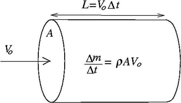
To understand the power contained in the wind one can consider an area normal to the wind velocity as shown in Fig. 9.1. After a time Δt the volume of air particles that has passed this area is ![]() , (where A is the cross-sectional area and Vo is the velocity) weighing
, (where A is the cross-sectional area and Vo is the velocity) weighing ![]() (where ρ is the density) and having a kinetic energy
(where ρ is the density) and having a kinetic energy ![]() and thus the available power (energy per time) in the wind is
and thus the available power (energy per time) in the wind is ![]() . The available power is thus proportional to the density of the air, the rotor area, and very importantly the wind speed cubed, and it is the purpose of any wind turbine to transform as cheap as possible some of this into useful power.
. The available power is thus proportional to the density of the air, the rotor area, and very importantly the wind speed cubed, and it is the purpose of any wind turbine to transform as cheap as possible some of this into useful power.
9.2 A Short Description on How a Wind Turbine Works
To comprehend the equations used to compute the aerodynamic loads on a wind turbine rotor it is very useful first to learn how a wind turbine basically works. It is clear that a device is needed that will slow down the wind speed in order to extract kinetic energy from the air and at the same a torque must be created that eventually can drive an electrical generator. Both can be accomplished by a few spinning blades having cross sections shaped as conventional airfoils as shown in Fig. 9.2.

The upper part of Fig. 9.2 shows the rotor seen from the front and the lower part displays the unfolded cut in the rotor plane at the radial position, r, indicated by the dashed line and seen directly from above. The first thing to note in the lower part of Fig. 9.2 is that the wind speed approaching the rotor has been reduced by a factor a·Vo, so that the apparent wind at the rotor plane is (1−a)Vo. The in-plane velocity is mainly the rotational speed of the blade at the radial distance r from the rotor axis, ωr, (where ω is the angular velocity of the rotor) but also a small extra contribution, a′ωr, is present, so that the effective tangential velocity experienced by the rotor is (1+a′)ωr. The two nondimensionalized velocities, a, and, a′, are called the axial- and the tangential induction factors, respectively, and if they were known, the relative wind, Vrel, approaching the rotor plane can be drawn in the so-called velocity triangle, see the lower left sketch in Fig. 9.2. By definition the lift is perpendicular and the drag parallel to the relative velocity as sketched in Fig. 9.2. The net aerodynamic loading is the vector sum of the lift and drag and denoted, R, in the figure and is the integral of the pressure and skin friction distribution on the airfoils at this radial position. It is seen that this resulting aerodynamic load vector has a component into the wind, pn, and an in-plane component, pt. The in-plane component, pt, delivers the required torque to the shaft and the normal loading provides a contribution to the necessary thrust force that is reducing the wind speed in order to extract power from the wind. It is also, pn, and, pt, that are responsible for the induced wind speeds a·Vo and a′·ωr, since these are the reactions on the wind velocity from the blade loadings. This ends the qualitative description of how a wind turbine works and next will be shown how the aerodynamic loadings and induced velocities can be quantitatively determined and thus eventually be used as a design tool.
9.3 1D Momentum Equations
The 1D momentum theory goes back more than 100 years and was developed by Froude and Rankine and is therefore often called the Rankine–Froude theory. The theory was originally developed for marine propulsion, but will be shown here for a wind turbine rotor. The rotor is modeled as a permeable disc with a normal load equally distributed over the rotor plane giving rise to a constant velocity profile in the wake. The integral of the normal loading can be integrated into one thrust force, T, as shown in Fig. 9.3. Only the flow confined by the streamlines touching the rotor tip is affected by the thrust force and the free wind speed upstream is gradually being reduced to a lower value in the wake, as sketched in Fig. 9.3.

It is seen in Fig. 9.3 that the velocity due to the thrust force, T, is decreasing with the downstream distance and since the mass flow is the same at any downstream plane the streamlines have to expand. The undisturbed wind speed is denoted Vo, the reduced velocity in the rotor plane is u and the velocity in the wake is u1. According to Section 9.2 the velocity in the rotor plane u may also be written as u=(1−a)Vo. Since there is no flow across the lateral streamlines touching the rotor tip the conservation of energy assuming no loss for the control volume confined by these are easily determined as
(9.1)
where ρ is the density of the air, A the rotor area, and P the power extracted from the wind. In deriving Eq. (9.1) is assumed that the pressure at the outlet has recovered to the ambient pressure, since the streamlines are now parallel again and also that none of the mechanical energy is dissipated into heat. Furthermore, one may apply the Bernoulli equation along the streamline from 1 to 2 and again from 3 to 4 as indicated in Fig. 9.3.
(9.2)
 (9.2)
(9.2)
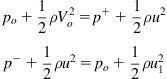
where po denotes the ambient pressure, p+ the pressure just upstream of the rotor, and p− the pressure just behind the rotor. These equations may be combined to
(9.3)
where Δp is the pressure drop over the rotor disc. Next a cylindrical control volume totally enclosing the flow through the rotor is considered as drawn by the dashed line in Fig. 9.4. Since the lateral boundary of this control volume is horizontal the pressure around the control volume can only contribute to an axial force at the in- and outlet planes, and here the pressure is assumed to be the ambient value. Therefore the net pressure force is zero and the only remaining force in the flow direction is the unknown thrust force, T. The lateral boundaries are no longer streamlines so there is a mass flow crossing the lateral boundaries of the control volume and that is carrying axial momentum. The conservation of axial momentum thus becomes
(9.4)

And combining this with the conservation of mass
(9.5)
Yields
(9.6)
Now since the thrust can also be expressed as the pressure drop over the rotor disc times the area the combination of Eqs. (9.3) and (9.6) gives:
(9.7)
Since by definition u=(1−a)Vo Eq. (9.7) gives that the velocity in the wake becomes u1=(1−2a)Vo and if this is introduced into Eq. (9.1) the power can written as:
(9.8)
The power is often nondimensionalized with the available power in the wind into the so-called power coefficient
(9.9)
And introducing Eq. (9.8) into (9.9) a simple expression is derived for an ideal power coefficient, Cp, assuming 1D flow and no losses
(9.10)
It is seen that the maximum value of Eq. (9.10) is Cp=16/27≈60% and occurs for a=1/3. This is known as the Betz limit and is an upper theoretical value for the power coefficient of a wind turbine.
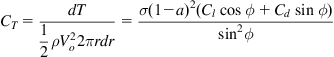
Also a thrust coefficient, CT, is defined as:
(9.11)
And it can be shown that using the definition of the axial induction factor and Eqs. (9.6) and (9.7) that the thrust coefficient for an ideal rotor becomes
(9.12)
The value of the thrust coefficient giving the theoretical maximum power coefficient is thus CT=8/9.
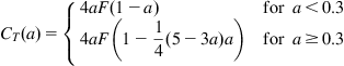
Even though a real rotor is not ideal and cannot be modeled as simple as a permeable disc, the Eqs. (9.10) and (9.12) still tell us something about the maximum that can be achieved; this happens for a thrust force giving an axial induction factor of approximately a=1/3. Measurements verify that Eq. (9.12) is valid up to approximately a=1/3 and for higher values of the axial induction factor an empirical correlation called the Glauert correction is used, and one often used expression is:
(9.13)
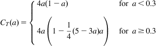 (9.13)
9.4 Blade Element Momentum Method
The blade element momentum (BEM) method as described by Glauert [1] is a generalization of the momentum theory coupled to the blade element theory often attributed to Drzewiecki. The blade element theory is that the flow past a given section is considered 2D and that the effective inflow velocity can be constructed as the vector sum of the incoming velocity and the rotational speed. However, when doing this one must also, as was shown by Glauert, include the induced velocities that are the reaction on the incoming flow from the aerodynamic blade loads. When doing this one can draw the so-called velocity triangle as shown in Fig. 9.5, where the induced velocity is included as W, and where the axial component is given as aVo (consistent with the 1D momentum theory) and the tangential component as a′ωr. Provided that the induced velocity is known, one can calculate the size and direction of the relative velocity. Assuming locally a 2D flow past an airfoil and that the lift and drag coefficients are available as a function of angle of attack and the Reynolds number, the lift and drag can be calculated as will be shown later. The problem left is then to estimate the induced velocities that are in equilibrium with the aerodynamic loads, and this is exactly what the BEM theory does.

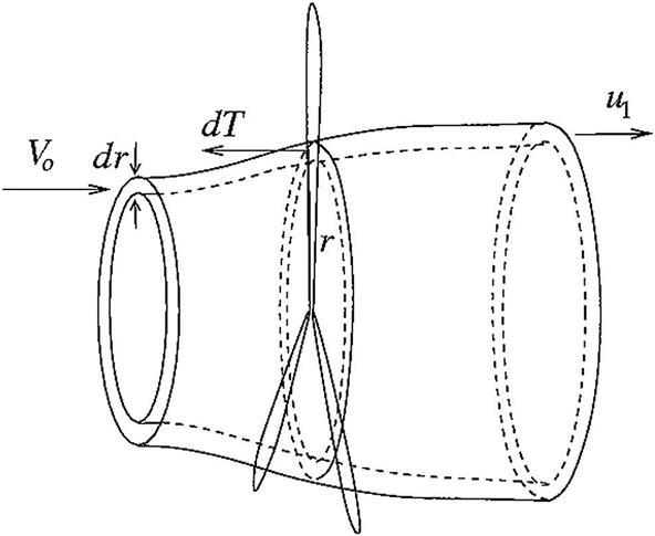
In BEM the loads and induced wind speeds are computed at a finite number of radial positions also denoted as elements. Furthermore, it is assumed that these elements are independent. A streamtube with thickness, dr, around each element is considered as shown in Fig. 9.6. The two lateral sides are assumed to be made up of streamlines and the partly empirical Eq. (9.13) is presumed also to be valid for the streamtube in Fig. 9.6. Furthermore, it is assumed that there are no azimuthal variations of the velocities at the outlet, u1, and in the rotor plane, u, which is only true if the thrust is also azimuthally constant corresponding to an infinite number of blades. A correction to this, denoted Prandtl’s tip loss correction, is introduced later. But for the moment the equations are derived as if the aerodynamic loads are distributed evenly at the area of the strip cutting the rotor plane dA=2πrdr. The thrust from one blade can be estimated from the blade element at the same radial position, r, from Fig. 9.7.

Provided that the axial and tangential induction factors, a and a′, are known the angle of the incoming relative wind with the rotor plane, ϕ, called the flow angle (Fig. 9.7) can be computed as:
(9.14)
And the size of the relative wind speed as
(9.15)
Knowing the angle between the rotor plane and the airfoil chord, θ, the local angle of attack is
(9.16)
The lift and drag coefficients are then found by a table look-up, Cl(α, Re) and Cd(α, Re), for the airfoil applied at this radial position, and from these the lift and drag (in units of N m−1) can be computed as:
(9.17)
 (9.17)
Next, these aerodynamic loads are projected normal (see also Fig. 9.7) and tangential to the rotor plane as
(9.18)
Finally, the thrust force at the streamtube in Fig. 9.6, can be calculated as
(9.19)
since pn multiplied by dr is the force from one blade and B being the number of blades. Eq. (9.19) is nondimensionalized as in the definition for the thrust coefficient Eq. (9.11), but using the strip area of the streamtube intersecting the rotor plane and using Eqs. (9.18) and (9.17) to determine the normal load and introducing the solidity, σ=Bc/2πr
(9.20)
 (9.20)
One can also apply the conservation of angular momentum for the control volume in Fig. 9.6 to find a relationship between a′ and the torque from the aerodynamic loads noting that the angular velocity upstream of the rotor is 0 and 2a′ωr in the wake
(9.21)
The torque can also be found directly from the tangential loads as:
(9.22)
Note that Ct in Eq. (9.22) is not the thrust coefficient but the tangential force coefficient given as:
(9.23)
From Eqs. (9.21) and (9.22) an expression for the tangential induction factor is derived
(9.24)
 (9.24)
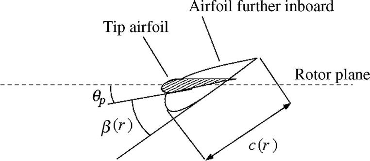
To describe the blade geometry one needs to have at some discrete radial positions (typically around 10–15 stations) the chord, c(r), the twist, β(r), and a table with the lift and drag coefficients as function of angle of attack. The chord, c(r), is the local width of the blade, the pitch, θp, is the angle between the rotor plane and the tip airfoil and the twist the angle between a local airfoil along the blade and the tip airfoil as shown in Fig. 9.8.
The angle between one blade element and the rotor plane θ in Eq. (9.16) is thus given as:
(9.25)
To evaluate the momentum equations from the control volume in Fig. 9.6, it has been assumed that there is no azimuthal variation of the induced velocities at the outlet, which would only be true for a rotor with infinite number of blades. Prandtl made a correction to the aerodynamic loads evaluated from the velocity triangle as in Fig. 9.7, so that when these are used for a rotor with infinite number of blades one gets approximately the same induction as for the real rotor with B blades. Prandtl evaluated the induced velocities from a lifting line model, where the blades are modeled as lines with a bound circulation distribution along the span. The local bound circulation can be estimated from Kutta–Joukowski theorem and the definition of the lift coefficient as:
(9.26)
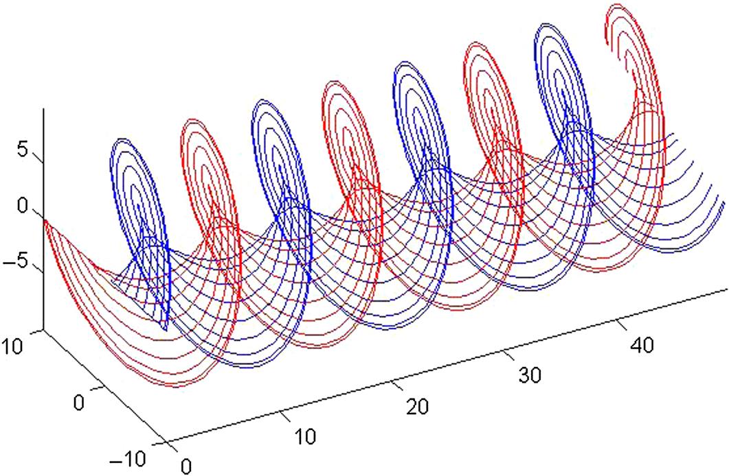
Next, there are vortices trailing from the blades and lying in a helical path as shown in Fig. 9.9 for a two-bladed rotor. The strength of the trailed vortices is given as the gradient of the bound circulation according to Helmholtz theorem. The only free parameter is then the helical pitch angle of the trailed vortex lines that must be specified, since the resulting induced velocities on the blades from this vortex system is a function of this pitch. But for a lightly loaded rotor the pitch can be approximated from the free wind speed and the angular velocity only. Knowing the geometry and the strength of the vortex lines the induced velocity, W, can be computed on the blades using Biot–Savart law for every vortex line:
(9.27)
where Γ is the circulation of one vortex line, ds, a small piece of the line with direction tangent to the line, and r the radius vector from that small piece to the point where the induced velocity is evaluated.
Prandtl solved this system using potential flow and a simple assumption of the wake geometry and came up with a correction to the loads, so that the induction at the blades become the same as a rotor with an infinite number of blades. The loads from the velocity triangle shown in Fig. 9.7 is divided by a factor, F, denoted by Prandtl’s tip loss correction, to model a system with an infinite number of blades that gives approximately the same solution as the vortex system shown in Fig. 9.9 for a finite number of blades. Then one can apply these loads to the momentum equations derived for an infinite number of blades:
(9.28)
where R is the rotor radius, r the local radius, and ϕ the local flow angle. When this correction is applied to the momentum equations (9.13) and (9.24) these become:
(9.29)
 (9.29)
and
(9.30)
 (9.30)
Now one has finally, all the equations needed to calculate the aerodynamic loads on a wind turbine rotor for a given blade geometry.
9.4.1 The Blade Element Momentum Method
The necessary input for the BEM method is as follows. First one has to decide the number of elements, typically 10–15, and their radial positions. The airfoil data in the form of lift and drag coefficients at each station as function of angle of attack and possibly the Reynolds number, must be obtained. Furthermore, the chord and twist must be known at the elements. With the geometry given, one must also define the operational parameters in the form wind speed Vo, pitch angle θp, and rotational speed ω.
1. Guess a value of the induction factors, a and a′
2. Calculate flow angle ϕ using Eq. (9.14)
3. Calculate angle of attack using Eqs. (9.16) and (9.25)
4. Determine lift and drag coefficients from tabulated airfoil data
5. Calculate Prandt’s tip loss factor Eq. (9.28)
6. Calculate thrust coefficient using Eq. (9.20)
7. Calculate new value of axial induction factor anew from Eq. (9.29)
8. Calculate tangential force coefficient using Eq. (9.23)
9. Solve Eq. (9.30) for a new value of the tangential induction factor a′new
10. Compare the new values of a and a′ with the values from previous iteration and if |anew−aold|<ε stop else go back to Step (2) and calculate a new flow angle, etc.
The BEM method described above is the classical one derived by Glauert [1], and is sufficient for blade design. But for unsteady load estimation this must be complemented by more submodels to handle the dynamic response of the induced wind to time-varying loads from the angle of attack changing due to, e.g., atmospheric turbulence, tower passage, and wind shear. To read more about this is referred to textbooks such as Hansen [2], Manwell et al. [3], Burton et al. [4], and Schaffarczyk [5].
9.5 Use of Steady Blade Element Momentum Method
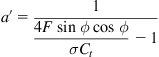
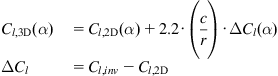
The BEM method can be used to analyze a given rotor design by computing the loads for varying operational parameters: angular velocity ω, pitch angle θp, and wind speed Vo. On a stall controlled wind turbine the blades are rigidly mounted to the hub and the pitch angle is thus constant. Further, an asynchronous generator is typically used where the rotational speed is almost constant, leaving only the wind speed as a free parameter. Fig. 9.10 shows the measured and computed power as function of wind speed for the Tellus 100 kW. The geometry for this rotor is reported in Schepers et al. [6]. It is seen that for low wind speeds where the angles of attack are also low and the local flow attached there is a very good agreement between the measured and computed power using 2D airfoil data. However, when using pure 2D airfoil data the flow seems to stall too early with a resulting underestimation of the power at high wind speeds, and to improve the numerical results one must correct the 2D airfoil data in stall using a stall delay model that takes into account the effects of rotation on the stalled boundary layer. The model used here is found in Chaviaropoulos and Hansen [7] and alters the lift coefficient as:
(9.31)
 (9.31)
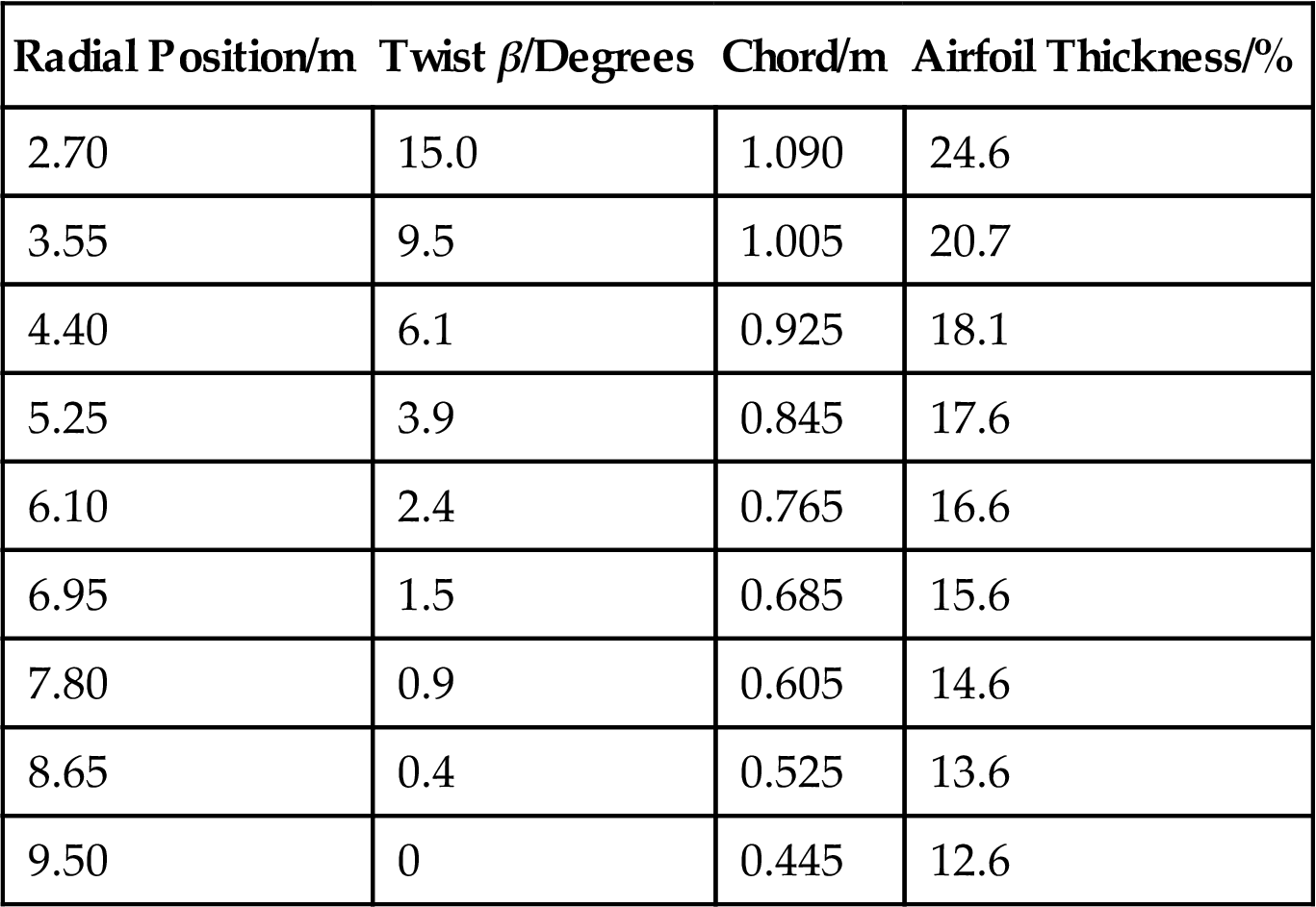
where r is the radial distance to the rotational axis, c the chord, and Cl,inv the inviscid lift coefficient. It should also be mentioned that the correction is only applied up to deep stall, where the 2D data are again applied. The Tellus turbine is a relatively small rotor with a radius of only 9.5 m and the rotational effects are thus stronger than on larger wind turbines, where the term (c/r) becomes small at the outer part of the blades. The overall blade data for the Tellus turbine is shown in Table 9.1 and the NACA 63 n-2nn airfoil is used, where the two last digits denote the thickness. 2D airfoil data can be found in airfoil catalogues, but are given in Ref. [6] for thicknesses 12, 15, 18, 21, and 25 and to find the actual airfoil data for a given thickness one has to interpolate between these 5 thicknesses. The rotational speed is 47.5 revolutions per minute (RPM) and the pitch angle is θp=−1.5 degrees.

Table 9.1
Global Blade Data for the 100 kW Tellus Wind Turbine as Described in Ref. [6]
| Radial Position/m | Twist β/Degrees | Chord/m | Airfoil Thickness/% |
| 2.70 | 15.0 | 1.090 | 24.6 |
| 3.55 | 9.5 | 1.005 | 20.7 |
| 4.40 | 6.1 | 0.925 | 18.1 |
| 5.25 | 3.9 | 0.845 | 17.6 |
| 6.10 | 2.4 | 0.765 | 16.6 |
| 6.95 | 1.5 | 0.685 | 15.6 |
| 7.80 | 0.9 | 0.605 | 14.6 |
| 8.65 | 0.4 | 0.525 | 13.6 |
| 9.50 | 0 | 0.445 | 12.6 |
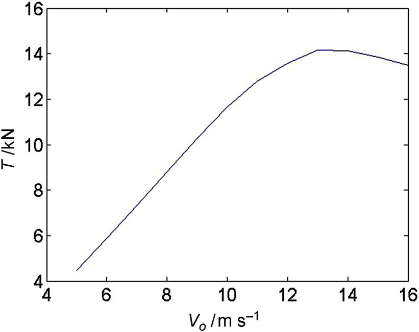
In Fig. 9.11 is shown the computed thrust force as function of wind speed for the stalled regulated Tellus wind turbine and it is seen that the thrust force increases with wind speed and stays high in high wind speeds, and in Fig. 9.12 is plotted the computed power and thrust coefficients. From Fig. 9.12 is seen that this wind turbine runs most efficiently between 6 and 9 m s−1, where Cp is around 0.44.
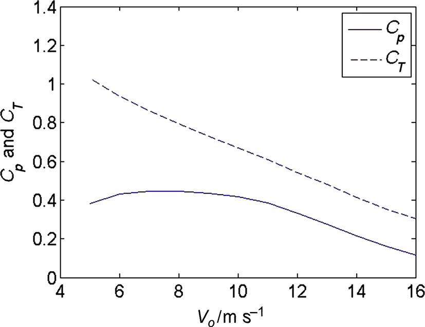
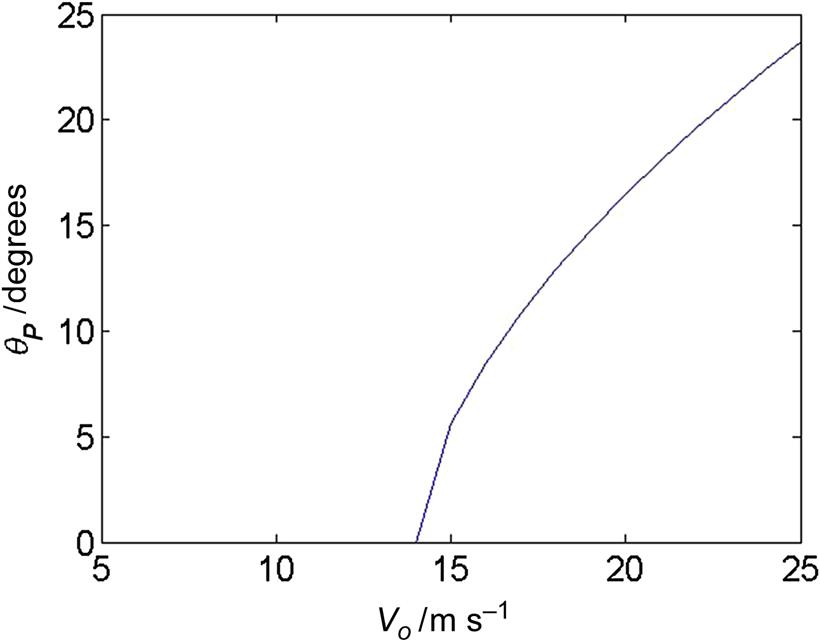
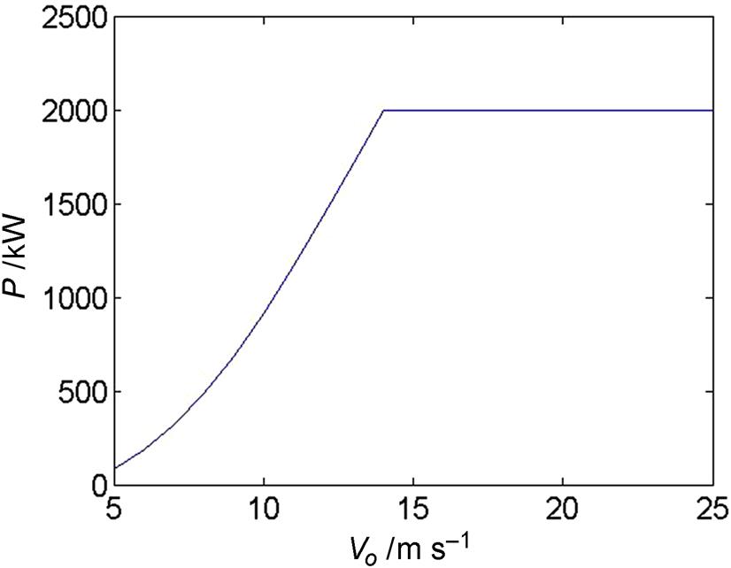
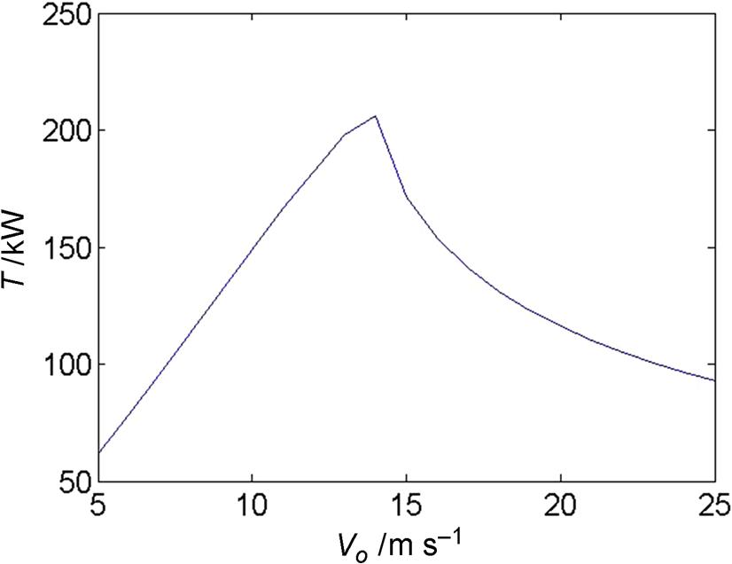
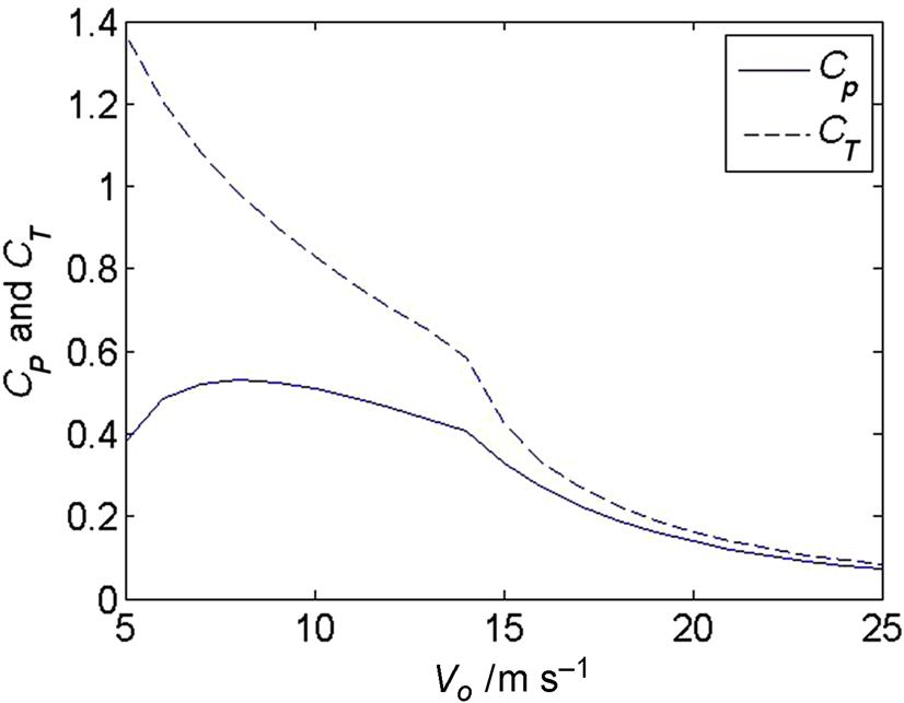
Many large wind turbines are pitch regulated, where the entire blades can be pitched to alter the angles of attack along the blade and thus also the loads. An example of a pitch regulated wind turbine is the 2 MW Tjaereborg wind turbine as described in Hau et al. [8]. The blades are NACA44xx airfoils and the overall rotor geometry is summarized in Table 9.2. Again airfoil data are found in airfoil catalogues as, e.g., Abbott and Doenhoff [9] and then interpolated in thickness for a specific element. The nominal rotor speed at rated power is 22.36 RPM and the pitch can vary between −2 and 35 degrees. Since the blades are pitched when reaching rated power of 2 MW the amount of stall is small and there is no need to correct the airfoil data for 3D rotational effects. With the BEM code it is possible to compute the necessary pitch to exactly keep the rated power at high wind speeds by varying the pitch until it is reached (Fig. 9.13) and the corresponding power and thrust curves are shown in Figs. 9.14 and 9.15. Note that the thrust first increases with wind speed but starts to decrease as soon as the blades are pitched toward lower angles of attack. Even though the Tjaereborg rotor is pitch regulated it is still only operating most efficiently at one wind speed (Cp,max=0.5 at Vo=8 m s−1) as shown in Fig. 9.16, where the power and thrust coefficients are plotted against wind speed.
Table 9.2
Global Blade Data for the 2 MW Tjaereborg Wind Turbine as Described in Ref. [8]
| Radial Position/m | Twist β/Degrees | Chord/m | Airfoil Thickness/% |
| 6.46 | 8.0 | 3.3 | 30.58 |
| 9.46 | 7.0 | 3.0 | 24.10 |
| 12.46 | 6.0 | 2.7 | 21.13 |
| 15.46 | 5.0 | 2.4 | 18.70 |
| 18.46 | 4.0 | 2.1 | 16.81 |
| 21.46 | 3.0 | 1.8 | 15.46 |
| 24.46 | 2.0 | 1.5 | 14.38 |
| 27.46 | 1.0 | 1.2 | 13.30 |
| 28.96 | 0.5 | 1.05 | 12.76 |
| 30.46 | 0.0 | 0.90 | 12.22 |

Modern wind turbine can further vary the angular velocity within a certain range. And assuming that for a given wind turbine the power depends on the air density, the viscosity, the wind speed, the rotor radius, the angular velocity, and the pitch angle as
(9.32)
one can derive that
(9.33)
The first parameter is the Reynolds number and this effect is small for large rotors and the second parameter is called the tip speed ratio λ. There is thus one combination of the tip speed ratio and pitch angle (λopt,θp,opt) that for a given design gives the highest possible power coefficient, and requires that the rotational speed varies as
(9.34)
and that the pitch angle is kept at θp,opt. Then the wind turbine will run at the highest possible efficiency for all wind speeds. However, this is in practice only possible up to a certain wind speed, since the rotational speed from Eq. (9.34) will become too large, so that the tip speed exceeds approximately 80–90 m s−1 where the aerodynamic noise becomes unacceptable. For such a turbine the power and thrust coefficients will be constant at their optimum value for the lower wind speeds and then start to decrease similar to Fig. 9.16, when the optimum tip speed ratio no longer can be kept as required by Eq. (9.34).
9.6 Aerodynamic Blade Design
Before describing a blade design process and how the BEM method can be used one needs first to define a good design. The object of any wind turbine related project is to reduce the price of producing 1 kW h considering the overall costs over the entire lifetime. To do this one must have a reliable cost model including, e.g., materials, manufacturing, and operation and maintenance cost, which is outside the scope of this chapter. Instead focus will be purely on obtaining an aerodynamically efficient rotor producing as many kWh m−2 a−1 (where a refers to annum) as possible, assuming this will also be the most economically profitable design. The actual design depends whether the turbine is stall regulated, pitch regulated, or variable speed pitch regulated. But in all cases one must combine the power curve P(Vo), with a given site-specific wind distribution h(Vo), where h is the actual annual number of hours in the wind speed interval Vo±0.5 m s−1. The total annual energy production is the sum of ∑h·P (in units of kW h) for all wind speed intervals between start and stop. Especially for a stall-regulated wind turbine the actual design will depend strongly on the actual wind distribution at a given site. First one must decide on a rotor radius and the airfoils. Today there exist airfoils specifically designed for wind turbine blades as, e.g., the Risø-A1 (fixed rotor speed, stall, or pitch), Risø-B1 (variable speed and pitch control), and Risø-P (pitch regulated, variable, or constant rotor speed) families, see Ref. [10]. The shape of these airfoils were described by only a few degrees of freedom, DOFs, and a fifth order B-spline and the optimum values for the DOFs were found using a Simplex method optimizing various object functions, depending on whether the airfoil is to be used at the root, the mid, or tip of the blade. The aerodynamics for a given set of DOFs was determined using the XFOIL code [11]. The important properties for a wind turbine airfoil are summarized and prioritized in Table 9.3 (inspired by Fuglsang and Bak [10]) depending on its radial placement. It is clear that the main purpose of the root sections is to carry high bending moment and therefore the structural properties are most important, and hence the high thickness to chord ratio. However, also the geometrical compatibility is important, since these airfoils must morph smoothly with the geometries at the mid and tip part of the blade. At the outer part of the blade contributing mostly to the thrust and power production the aerodynamic properties such as high lift, high lift to drag ratio, benign poststall behavior, low roughness sensitivity and low noise are all very important. And the airfoils at the mid part of the blades should be able to both carry loads and produce power and be geometrically compatible with the root and tip airfoils. It is very important to verify the designs found using preferably both Computational Fluid Dynamics (CFD) and wind tunnel experiments, since XFOIL is based on the integral boundary layer equations not fully valid after stall, and therefore especially the real poststall behavior may be different. Further, it is possible to cure some of the bad aerodynamic properties of the thick root airfoils by applying vortex generators and Gourney flaps, see Ref. [12].
Table 9.3
Relative Importance of Airfoil Properties
| Root | Mid Part | Tip | |
| Thickness to chord ratio/% | >27 | 21–27 | 15–21 |
| Structure | +++ | ++ | + |
| Geometrical compatibility | ++ | ++ | ++ |
| Maximum roughness insensitivity | + | +++ | |
| High max lift coefficient | + | +++ | |
| Benign post stall behavior | + | +++ | |
| Low aerodynamic noise | +++ |

Now having decided on the airfoils one can start to think about how to design a good blade with respect to chord and twist distribution. The easiest and most straightforward design is a so-called one-point design, where the blade layout is calculated to obtain the highest possible power coefficient for one specific tip speed ratio and pitch angle. Since the BEM assumes that the different elements along the blade are independent they can be individually optimized to maximize the local power coefficient at each element, dCp, defined as
(9.35)
And can be combined with Eq. (9.22) to give
(9.36)
The input to the design is a specified rotor radius, R, a given tip speed ratio, λ, and given airfoils along the blade. The design angle of attack, αd, is for the radial element the one giving the highest lift to drag ratio and thus fixed. That means that also the lift and drag coefficients are fixed corresponding their value at the design angle of attack. Now for every radial position following algorithm is made for various chord lengths.
6. Update a and a′ using Eqs. (9.29) and (9.30)
7. Check convergence, if not go back to Step (2) with new values of a and a′
8. Calculate dCp(c/R) using Eq. (9.36)
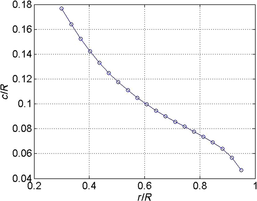
Pick the value giving the highest local power coefficient and also note the local pitch, θ(r), and chord, c(r) and continue with the next element. In Figs. 9.17 and 9.18 are shown the result using this one-point optimization for following parameters λ=6, B=3, αd=4, Cl=0.8, and Cd=0.012. The overall power coefficient for this design is 0.44, which is not impressive and can be improved by choosing more efficient airfoils with less drag, especially for the outer part of the blade.

One could further improve the one-point design by slightly adjusting locally the twist angle at every element to maximize energy production in a wind speed interval, between 6 and 9 m s−1 where most energy is typically produced. To do so one can for each section calculate, using a BEM code, the local power production (kW m−1) as function of twist angle and wind speed as
(9.37)
Next the produced energy in the chosen wind speed interval as function of twist angle is computed, ![]() (kW h m−1 a−1) (where a refers to annum) by combining the local power production with the annual number of hours in each wind speed interval as described earlier, and the twist angle producing most energy per meter blade is finally adopted.
(kW h m−1 a−1) (where a refers to annum) by combining the local power production with the annual number of hours in each wind speed interval as described earlier, and the twist angle producing most energy per meter blade is finally adopted.
An alternative one-point optimization would be to replace the BEM code with a lifting line using Eqs. (9.26) and (9.27) and letting the trailed vortex lines follow a helical pitch as shown in Fig. 9.9 and requiring that the axially induced velocity along the rotor blades should be constant. This would, however, give something very close the one-point optimized blade using the BEM equations, since these have been calibrated through Prandtl’s tip loss correction to give approximately the same as this vortex model. Doing this, one should change the pitch of the helical wake iteratively as a function of the computed induction.
For a more complete optimization one could still use the BEM code to calculate the power and thrust as function of the rotational speed, the wind speed, the pitch angle, and the chord and twist distribution. The chord and twist distribution is then typically described by a limited number of DOFs, e.g., a spline and the BEM model is coupled to a formal optimization algorithm as, e.g., the Simplex method finding the geometry and operational parameters that maximizes the annual energy yield under certain constrains for a given wind distribution.
9.7 Unsteady Loads and Fatigue
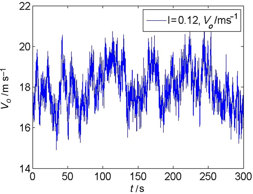
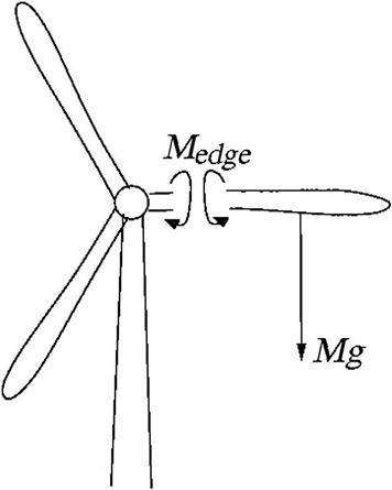
A big challenge for a wind turbine is that the loads are inherently unsteady, mainly due to atmospheric turbulence and gravity. The wind speed in one fixed point in space is constantly due to atmospheric turbulence fluctuating around a mean value as, e.g., shown in Fig. 9.19 for a mean wind speed of Vo=18 m s−1 and a turbulence intensity of I=σ/Vo=12%. When a wind turbine blade spins around in a turbulent wind field, both the size and direction of the wind velocity in the velocity triangle drawn in Fig. 9.7 is changing in time and thus also the aerodynamic loads. Furthermore, gravity gives a large one per revolution periodic load mainly in the edgewise direction of a blade, as indicated in Fig. 9.20. Other unsteady loads come from wind shear, tower passage and if the rotor in a wind farm is partly in the wake of an upstream turbine. Wind shear is when the wind speed increases with height so that the apparent wind speed is higher at the top position than when a blade half a revolution later is pointing down, and this gives a sinusoidal variation with the frequency of the rotation. The time it takes for a blade to pass the tower is small, but during this time the wind speed is reduced giving a sudden drop in the loads that acts as an impulsive loading.
Further, the blades will respond elastically to the time-varying loads and the velocities from the vibrations also change the angles of attack and to solve for the time-dependent loads and deflections one needs to calculate in the time domain the coupled structural- and aerodynamic problem using a so-called aeroelastic code. To reduce the risk of a blade failure different norms exist, e.g., IEC 61400-3 that describe the load cases that a wind turbine is expected to experience during its design lifetime including: normal operation, extreme situations such as extreme wind and wave situations, fault conditions, starts and stops, etc. Each of these load cases must for a given design be simulated in time and the accumulated fatigue damage weighted with the expected occurrence of the various load cases must not lead to failure and also it must be checked that the ultimate loads do not cause any structural damage.
9.8 Brief Description of Design Process
A typical design process will then be something like this. First, the wind turbine is designed combining a simple aerodynamic model as described in the previous sections with an optimization algorithm, where the object is to minimize the LCoE. Now for this design all the load cases described in the standards are then simulated aeroelastically in the time domain including the structural response to the time-varying loads and the extreme and fatigue loads are input to more advanced structural models, such as Finite Element Models (FEM), for the various components used in the turbine. If these FEM-based calculations reveal some structural problems one has to go back and change the design and redo all the cases to make new load input to the structural models, and so on until one believes to have an optimized design that with a very high probability will survive all the expected dynamic loads experienced during the entire design lifetime. Now, typically also the final blade design is checked using advanced flow solvers such as CFD codes to verify the aerodynamic loads found using the simpler models relying on tabulated airfoil data. And now the design has to physically be built and tested before it is allowed to be erected outside test stands and sold commercially.