
Economics of Wind Power Generation
Magdi Ragheb, University of Illinois at Urbana-Champaign, Urbana, IL, United States Email: [email protected]
Abstract
A discussion of the economics of wind power generation is presented. Sustainable development will depend on whether energy prices of other sources will stay high. Developers of wind power installations are looking at a 20-year investment span. If natural gas prices fall over that period, a project that is presently profitable could become uncompetitive a few years into the future. The growth is driven by tax incentives, utility demand, falling costs, and improved technology, including taller towers and lighter rotor blades.
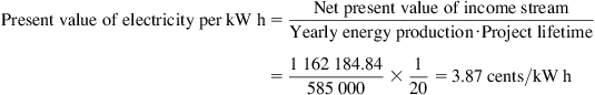
A benchmark calculation of the levelized cost of wind power electricity is presented. The effect of subsidies in the form of the production tax credit (PTC) is considered, and then the depreciation, taxes payments are incorporated into the calculation model. Compared with a benchmark calculation, the PTC can be inferred to contribute a present value of 0.57 cent (kW h)−1 to the income stream from the produced electricity.
Transmission costs are a major issue in wind energy development. Some of the best locations for generating wind energy are far distant from the consuming industrial and population centers. A massive upgrade of the transmission lines nationwide through the national electrical power grid using high-voltage DC instead of high-voltage AC is needed to tap those distant sources. Where water supplies are abundant, along seashores or internal lakes or rivers, the electricity produced could be used for extracting hydrogen from water through the electrolysis process. Hydrogen then can become the storage medium and energy carrier of wind energy. It would be conveyed or transmitted to the energy consumption sites possibly through the existing natural gas pipeline system which covers the United States. Another alternative is to convert hydrogen with coal into methane gas, CH4 that could be distributed through the existing natural gas distribution grid without significant modifications. Methane itself can be converted into methanol or methyl alcohol, CH3OH as a liquid transportation fuel. To reduce the electrical transmission losses, one can envision superconducting electrical transmission lines cooled with cryogenic hydrogen carrying simultaneously electricity and hydrogen from the wind energy production sites to the consumption sites. Such a visionary futuristic power transmission system could also provide the electrical power for a modern mass transit system using magnetically levitated (Maglev) high-speed trains transporting goods and people supplementing the current highway system in the United States.
Keywords
Wind cost; wind economics; windmill; wind turbine; wind power generation; incentives; levelized cost; present value; PTC; ITC; REPI; intermittence factor
Everything on Earth belongs to princes, except the wind.
Victor Hugo, French author
25.1 Introduction
Wind energy capital costs have declined steadily. A typical cost for a typical onshore wind farm has reached around $1000 kW−1 of installed rated capacity, and for offshore wind farms about $1600 kW−1. The corresponding electricity costs vary due to wind speed variations, locations, and different institutional frameworks in different countries [1].
A symbiotic relationship is emerging between agricultural farming and electrical wind farming in the American Midwest. Landowners obtain attractive royalties from the installation of wind turbines on their land while continuing to farm around them; much like ranchers obtain royalties from oil and gas wells drilled on their cattle grazing properties. Each turbine uses an area of about 1–1.6 ha (2.5–4 acres) including the electrical cabling and access roads, while paying a royalty in the range of $5000–10000 per year per installed turbine. Small businesses with wind turbines installations can extract energy from the electrical grid, overcoming the intermittence property of the wind, and its surplus production; if not stored, can be wheeled into the electrical grid (Fig. 25.1).

25.2 Economic Considerations
A driver behind the growth in wind energy investment is the falling cost of wind-produced electricity. The cost of generating electricity from utility-scale wind systems has dropped by more than 80%. When large-scale wind farms were first set up in the early 1980s, wind energy was costing as much as $0.30 (kW h)−1 (30 cents per kilowatt-hour). New installations in the most favorable locations can produce electricity at less than $0.05 (kW h)−1, which is competitive to other energy sources (Fig. 25.2).

Fossil fuels such as petroleum, coal, and natural gas prices are helping to make wind power generation competitive. Even where wind power is still not able to compete head-on with cheaper power sources in some locations, it is getting close.
Continued investment will depend on whether energy prices of other sources will stay high. Developers of wind power installations are looking at a 20-year investment span. If natural gas prices fall over that period, a project that is now profitable could become uncompetitive a few years into the future. The growth is driven by tax incentives, utility demand, falling costs, and improved technology, including taller towers and lighter rotor blades [2, 3].
25.3 Wind Energy Cost Analysis
In generation technologies, the cost of electricity is primarily affected by three main components:
Wind power generation benefits from a fuel cost of zero. Studies of the cost of wind energy and other renewable energy sources could become unreliable because of a lack of understanding of both the technology and the economics involved. Misleading comparisons of costs of different energy technologies are common. The cost of electricity in wind power generation includes the following components:
25.4 Levelized Cost of Electricity
The levelized cost of electricity (LCOE) in electrical energy production can be defined as the present value of the price of the produced electrical energy (usually expressed in units of cents per kilowatt hour), considering the economic life of the plant and the costs incurred in the construction, operation and maintenance, and the fuel costs.
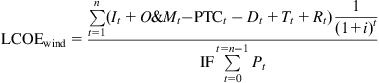
The fuel cost is zero in wind power generation, and the wind turbine is factory-assembled and directly delivered to the wind park site, resulting in a short construction time, t. This results in the following form for the LCOE for wind power generation, accounting for the intermittence factor IF, the production tax credit, PTCt, the depreciation credit Dt, the tax levy Tt, and the royalties or land payments Rt:
(25.1)
 (25.1)
where
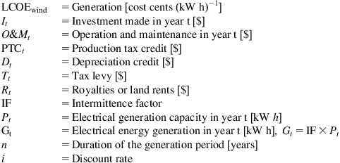
The present value factor (PVF) is:
(25.2)
The LCOE is estimated over the lifetime of the energy-generating technology, typically 20 years for wind generators. The discount rate (i) is chosen depending on the cost and the source of the available capital, considering a balance between equity and debt financing and an estimate of the financial risks entailed by the project.
25.5 Net Present Value
It is advisable to consider the effect of inflation, and consequently using the real interest rate r instead of just i. The net present value of a project is the value of all payments, discounted back to the beginning of the investment. For its estimation, the real rate of interest r defined as the sum of the discount rate i and the inflation rate s:
(25.3)
should be used to evaluate the future income and expenditures.
If the net present value is positive, the project has a real rate of return which is larger than the real rate of interest r. If the net present value is negative, the project has an unsustainable rate of return. The net present value is computed by taking the first yearly payment and dividing it by (1+r). The next payment is then divided by (1+r)2, the third payment by (1+r)3, and the nth payment by (1+r)n. Those terms are added together to the initial investment to estimate the net present value:
(25.4)
The electricity cost per kilowatt hour is calculated by first estimating the sum of the total investment and the discounted value of operation and maintenance costs in all years. The income from the electricity sales is subtracted from all nonzero amounts of payments at each year of the project period.
Depreciation is used in accounting, economics, and finance to spread the cost of an asset over the span of its productive life span. Depreciation is the reduction in the value of an asset or good due to usage, passage of time, wear and tear, technological outdating or obsolescence, depletion, inadequacy, rot, rust, decay, or other similar factors. Tax depreciation or accounting depreciation is sometimes confused with economic depreciation.
25.6 Straight Line Depreciation
Straight line depreciation is the simplest and most often used method in which we can estimate the real value of the asset at the end of the period during which it will be used to generate revenues, or its economic life. It will expense a portion of the original cost in equal increments over the period. The real value is an estimate of the value of the asset or good at the time it will be replaced, sold, or disposed of. It may be zero or even negative. Accordingly:
(25.5)
where a refers to annum or year.
25.7 Price and Cost Concepts
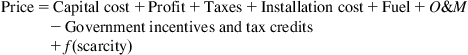
The words “cost” and “price” are sometimes mistakenly used as synonyms. The price of a product is determined by supply and demand for the product. Some people assume that the price of a product is somehow a result of adding a normal or reasonable profit to a cost, which is not necessarily the case unless it is applied to a government-managed monopoly. A factor that is a function of the scarcity of wind resources at a given location, as well as the taxes paid, could be accounted for; thus:
(25.6)
 (25.6)
25.8 Wind Turbines Prices
Wind turbine prices may vary due to the transportation costs, different tower heights, rotor diameters, generators capacities, and the grid connection costs. Some of the manufacturers’ deliveries are complete turnkey projects including planning, turbine nacelles, rotor blades, towers, foundations, transformers, switchgear, and other installation costs including road building and power lines. The manufacturer sales figures also include service and sales of spare parts.
The manufacturers’ sales include licensing income, but the corresponding rated power in units of megawatts is not registered in the company’s accounts. Sales may vary significantly between markets for high-wind resources turbines and low-wind resources turbines. The prices of different types of turbines are different. The patterns of sales, types of turbines, and types of contracts vary significantly from year to year and depend on the different locations and markets. A reasonable approach is to obtain the prices from the price lists and to consider the price in units of dollars per square meter of rotor swept area.
The operation and maintenance cost can be estimated as either a fixed amount per year or a percentage of the cost of the turbine. This could also include a service contract with the wind turbine manufacturer.
25.9 Intermittence Factor
The intermittence factor (IF), similar to the capacity factor (CF) for an energy-generating technology is equal to the ratio of the actual annual energy production to the rated maximum energy production, if the generator were running at its rated electrical power all year.
(25.7)
Depending on the wind statistics for a particular site, the practical intermittence factor for an onshore wind turbine is in the range of 25%–40%.
25.10 Land Rents, Royalties, and Project Profitability
In wind energy production, the land rents or royalties depend on the profitability of a project and not vice versa.
(25.8)
The compensation, land rents, or royalties paid to landowners where the turbines are located is sometimes treated as a cost of wind energy. In fact, it is only a minor share of the compensation which is a cost of the loss of crop on the area that can no longer be farmed; a possible nuisance compensation since the farmer has to make extra turns when plowing the fields underneath the wind turbines and he must be compensated for soil compaction and the damage to tiling from the heavy equipment access to the turbine site.
If the compensation exceeds what is paid to install a power line tower, the excess is an income transfer. It is not a cost to society, but is a transfer of income or profits from the wind turbine operator to the landowner. Such a profit transfer is called a land rent by economists. A rent payment does not transfer real resources from one use to another.
There is no standard compensation for placing a wind turbine on agricultural land. It depends on the quality of the site, the availability of the wind, and the grid access nearby. A landowner can bargain for a high compensation in a good location, since the turbine operator can afford to pay it due to the profitability of the site. If the site has low wind speed, and high installation costs, the compensation will be estimated closer to the nuisance value of the turbine.
25.11 Project Lifetime
The figure used for the design lifetime of a typical wind turbine is 20 years. It used to be a 30-year lifetime. With the low turbulence of offshore wind conditions leading to lower vibrations and fatigue stresses, it is likely that the turbines can last longer, from 25 to 30 years, provided that corrosion from salty conditions can be controlled. Offshore foundations for oil installations are designed to last 50 years, and it may be possible to consider two generations of turbines to be built on the same foundations, with an overhaul repair at the midlife point after 25 years.
25.12 Benchmark Wind Turbine Present Value Cost Analysis
An attempt is made at the estimation of a present value cost analysis for the cost of electricity over 20 years’ turbine project duration. A benchmark problem is first presented that could be later modified to accommodate other factors, such as the PTC, depreciation, and taxes [8].
25.12.1 Investment
Expected lifetime=20 a.
Turbine rated power: 600 kW.
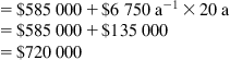
Turbine cost: $450 000
Installation costs: 30% of turbine price=$450 000×0.30=$135 000
Total turbine cost=Turbine cost+Installation cost
25.12.2 Payments
The payments, including the initial payment, are used to calculate the net present value and the real rate of return over 20 years’ project lifetime since this is the main economic aspect of the analysis. The tax payments and credits and the depreciation credits are not considered for simplification but could be added for a more detailed analysis later. We consider that the capital is in the form of available invested funds: if the capital cost is all borrowed funds, then the interest payment on the loan or the bonds must be accounted for.
Operation and maintenance: 1.5% of turbine price=0.015×450 000=6750 [$ a−1].
Total expenditure=Total turbine cost+Operation and maintenance cost over expected lifetime
25.12.3 Current Income and Expenditures per Year
Intermittence factor: 28.54%=0.2854.
Energy produced in a year: 600×365×24×0.2854=1 500 000 kW h a−1.
Price of electricity=$0.05 kW h−1.
Gross yearly income from electricity sale: 1 500 000 kW h a−1 at $0.05 (kW h)−1=1 500 000×0.05=$75 000 a−1.
Net income stream per year: $75 000 − $6750=$68 250 a−1.
One can construct Table 25.1 over the 20 years’ useful lifetime of the turbine.
Table 25.1
Benchmark Present Value Calculation for a 0.6 MW Rated Power Wind Turbine
| Number of Years | Expenditures/$ | Gross Income Stream/$ | Net Income Stream/$ | Present Value Factor 1/(1+r)n r=0.05 | Net Present Value of Income Stream/$ |
| 0 | −585 000 | – | – | – | – |
| 1 | −6 750 | 75 000 | 68 250 | 0.9524 | 65 000 |
| 2 | −6 750 | 75 000 | 68 250 | 0.9070 | 61 903 |
| 3 | −6 750 | 75 000 | 68 250 | 0.8638 | 58 957 |
| 4 | −6 750 | 75 000 | 68 250 | 0.8227 | 56 149 |
| 5 | −6 750 | 75 000 | 68 250 | 0.7835 | 53 475 |
| 6 | −6 750 | 75 000 | 68 250 | 0.7462 | 50 929 |
| 7 | −6 750 | 75 000 | 68 250 | 0.7107 | 48 504 |
| 8 | −6 750 | 75 000 | 68 250 | 0.6768 | 46 194 |
| 9 | −6 750 | 75 000 | 68 250 | 0.6446 | 43 995 |
| 10 | −6 750 | 75 000 | 68 250 | 0.6139 | 41 899 |
| 11 | −6 750 | 75 000 | 68 250 | 0.5847 | 39 904 |
| 12 | −6 750 | 75 000 | 68 250 | 0.5568 | 38 004 |
| 13 | −6 750 | 75 000 | 68 250 | 0.5303 | 36 194 |
| 14 | −6 750 | 75 000 | 68 250 | 0.5051 | 34 471 |
| 15 | −6 750 | 75 000 | 68 250 | 0.4810 | 32 829 |
| 16 | −6 750 | 75 000 | 68 250 | 0.4581 | 31 266 |
| 17 | −6 750 | 75 000 | 68 250 | 0.4363 | 29 777 |
| 18 | −6 750 | 75 000 | 68 250 | 0.4155 | 28 359 |
| 19 | −6 750 | 75 000 | 68 250 | 0.3957 | 27 009 |
| 20 | −6 750 | 75 000 | 68 250 | 0.3769 | 25 723 |
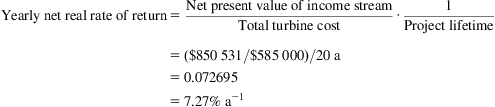
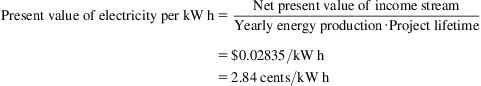
| Total | −720 000 | 1 500 000 | 1 365 000 | – | 850 531.5 |

From the table the net present value of income stream at r=5% a−1 real rate of interest: $850 531.5.
25.13 Incentives and Subsidies
25.13.1 Production Tax Credit (PTC)
In a measure taken by the US Congress a federal policy for promoting the development of renewable energy was initiated. The PTC provided initially a $0.015 kW h−1 (1.5 cents per kilowatt-hour) benefit for the first 10 years of a renewable energy facility’s operation. Originally enacted in 1992 the PTC has been renewed and expanded numerous times (Fig. 25.3). The USA FY16 Omnibus Appropriation Bill included a 5-year extension and phase-down of the PTC and the option to elect the Investment Tax Credit (ITC) for wind energy. The tax credits, extended through 2019, are phased-down by 20 percent each year beginning in 2017.

25.13.2 Investment Tax Credit (ITC)
Renewable energy facilities placed in service after 2008 and commencing construction prior to 2015 (or 2020 for wind facilities) may elect to make an irrevocable election to claim the investment tax credit (ITC) in lieu of the PTC. Projects that begun construction in 2015 and 2016 are eligible for a full 30 percent ITC, for 2017 a 24 percent, for 2018 an 18 percent, and for 2019 a 12 percent ITC. Wind facilities making such an election will have the ITC amount reduced by the same phase-down specified above for facilities commencing construction in 2017, 2018, or 2019. The Consolidated Appropriations Act 2016 (H.R. 2029 Section 301) extended both the PTC and permission for PTC-eligible facilities to claim the ITC in lieu of the PTC through the end of 2016 (and the end of 2019 for wind facilities) (Fig. 25.3).
25.13.3 Renewable Energy Production Incentive (REPI)
An incentive similar to the PTC is made available to public utilities, which do not pay taxes and therefore cannot benefit from a tax credit. The incentive is called the renewable energy production incentive (REPI) and it consists of a direct payment to a public utility installing a wind plant that is equal to the PTC at $0.015 kW h−1 (1.5 cents per kilowatt-hour) adjusted for inflation. Since the REPI involves the actual spending of federal funds, money must be “appropriated” or voted for it annually by the US Congress. It is sometimes difficult to obtain full funding for REPI because of competing federal spending priorities.
The American Wind Energy Association (AWEA) estimates that the investment in renewable systems could fall by as much as 50% without the PTC in place. This would wreak havoc with the energy investment cycle and all but shut many projects down. Losing the PTC would strangle the vendor base disrupt the work force and curtail future output.
Combined with a growing number of states that have adopted renewable electricity standards, the PTC has been a major driver of wind power development over the last years. Unfortunately the “on-again/off-again” status that has historically been associated with the PTC contributes to a boom-bust cycle of development that plagues the wind industry. The cycle begins with the wind industry experiencing strong growth in development around the country during the years leading up to the PTC’s expiration. Lapses in the PTC then cause a dramatic slowdown in the implementation of planned wind projects. When the PTC is restored the wind power industry takes time to regain its footing and then experiences strong growth until the tax credits expire.
Extending the PTC allows the wind industry to continue building on previous years’ momentum but it is insufficient for sustaining the long-term growth of renewable energy. The planning and permitting process for new wind facilities can take up to 2 years or longer to complete. As a result many renewable energy developers that depend on the PTC to improve a facility’s cost effectiveness may hesitate to start a new project due to the uncertainty that the credit will still be available to them when the project is completed.
25.14 Wind Turbine Present Value Cost Analysis Accounting for the PTC
We modify the calculation scheme for the benchmark problem to study the effect of the PTC on the present value of the produced electrical energy.
25.14.1 Payments
Installation costs: 30% of turbine price=$45 000×0.30=$135 000.
Total turbine cost=Turbine cost+Installation cost.
Operation and maintenance: 1.5% of turbine price=$.015×450 000=$6750 a−1.
Total expenditure=Total turbine cost+Operation and maintenance cost over expected lifetime.

25.14.2 Current Income and Expenditures per Year
Intermittence factor (28.54%)=0.2854.
Energy produced in a year: 600×365×24×0.2854=1 500 000 kW h a−1.
Gross yearly income from electricity sale: 1 500 000 kW h a−1 at $0.05 (kW h)−1=1 500 000×0.05=$75 000 a−1.
Yearly income from PTC of 1.5 cents (kW h)−1=1 500 000×0.015=$22 500 a−1 (over first 10 years of project).
Net income stream per year (first 10 years): $75 000 − $6750+22 500=$90 750 a−1.
Net income stream per year (next 10 years): $75 000 − $6750=$68 250 a−1 (Table 25.2).
Table 25.2
Benchmark Present Value Calculation for a 0.6 MW Rated Power Wind Turbine Accounting for the PTC Incentive
| Year n | Expenditures/$ | Gross Income Stream/$ | PTC/$ | Net Income Stream/$ | Present Value Factor 1/(1+r)n r=0.05 | Net Present Value of Income Stream/$ |
| 0 | −585 000 | – | – | – | – | – |
| 1 | −6 750 | 75 000 | 22 500 | 90 750 | 0.9524 | 86 430 |
| 2 | −6 750 | 75 000 | 22 500 | 90 750 | 0.9070 | 82 310 |
| 3 | −6 750 | 75 000 | 22 500 | 90 750 | 0.8638 | 78 390 |
| 4 | −6 750 | 75 000 | 22 500 | 90 750 | 0.8227 | 74 660 |
| 5 | −6 750 | 75 000 | 22 500 | 90 750 | 0.7835 | 71 103 |
| 6 | −6 750 | 75 000 | 22 500 | 90 750 | 0.7462 | 67 718 |
| 7 | −6 750 | 75 000 | 22 500 | 90 750 | 0.7107 | 64 496 |
| 8 | −6 750 | 75 000 | 22 500 | 90 750 | 0.6768 | 61 420 |
| 9 | −6 750 | 75 000 | 22 500 | 90 750 | 0.6446 | 58 497 |
| 10 | −6 750 | 75 000 | 22 500 | 90 750 | 0.6139 | 55 711 |
| 11 | −6 750 | 75 000 | – | 68 250 | 0.5847 | 39 904 |
| 12 | −6 750 | 75 000 | – | 68 250 | 0.5568 | 38 004 |
| 13 | −6 750 | 75 000 | – | 68 250 | 0.5303 | 36 194 |
| 14 | −6 750 | 75 000 | – | 68 250 | 0.5051 | 34 471 |
| 15 | −6 750 | 75 000 | – | 68 250 | 0.4810 | 32 829 |
| 16 | −6 750 | 75 000 | – | 68 250 | 0.4581 | 31 266 |
| 17 | −6 750 | 75 000 | – | 68 250 | 0.4363 | 29 777 |
| 18 | −6 750 | 75 000 | – | 68 250 | 0.4155 | 28 359 |
| 19 | −6 750 | 75 000 | – | 68 250 | 0.3957 | 27 009 |
| 20 | −6 750 | 75 000 | – | 68 250 | 0.3769 | 25 723 |
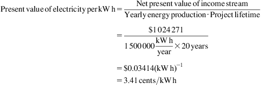
| Total | −720 000 | 1 500 000 | 225 000 | 1 590 000 | – | 1 024 271 |

The PTC pays fully 225 000/585 000=0.3846 or 38.46% of the initial cost of the turbine.
Net present value of income stream at r=5% a−1. Real rate of interest: $1 24 271.
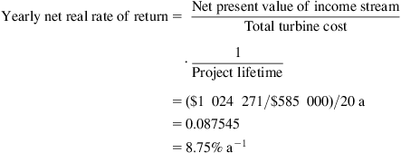
Compared with the benchmark calculation, the PTC can be inferred to contribute a present value of:
to the income stream from the produced electricity.
25.15 Accounting for the PTC as Well as Depreciation and Taxes
The owner of a wind power farm has to pay taxes for the incomes he is obtaining from the electricity sales. Assuming a 25% tax rate (Table 25.3).
Table 25.3
Benchmark Present Value Calculation for a 0.6 MW Rated Power Wind Turbine Accounting for the PTC Incentive as Well as Depreciation and Tax Payments
| Year | Expenditure/$ | Gross Income From Electricity Sale/$ | Tax 25% Gross Expenditure/$ | Linear Depreciation at 2.5% a−1/$ | PTC/$ | Net Taxes (Tax Depreciation)/$ | Net Income/$ | Present Value Factor | Net present value of income/$ |
| 0 | −585 000 | – | – | – | – | – | – | – | – |
| 1 | −6 750 | 75 003.12 | 17 063.28 | 14 625 | 22 500.936 | 2 438.28 | 101 815.776 | 0.952380952 | 96 967.41 |
| 2 | −6 750 | 75 003.12 | 17 063.28 | 14 625 | 22 500.936 | 2 438.28 | 101 815.776 | 0.907029478 | 92 349.91 |
| 3 | −6 750 | 75 003.12 | 17 063.28 | 14 625 | 22 500.936 | 2 438.28 | 101 815.776 | 0.863837599 | 87 952.29 |
| 4 | −6 750 | 75 003.12 | 17 063.28 | 14 625 | 22 500.936 | 2 438.28 | 101 815.776 | 0.822702475 | 83 764.09 |
| 5 | −6 750 | 75 003.12 | 17 063.28 | 14 625 | 22 500.936 | 2 438.28 | 101 815.776 | 0.783526166 | 79 775.32 |
| 6 | −6 750 | 75 003.12 | 17 063.28 | 14 625 | 22 500.936 | 2 438.28 | 101 815.776 | 0.746215397 | 75 976.50 |
| 7 | −6 750 | 75 003.12 | 17 063.28 | 14 625 | 22 500.936 | 2 438.28 | 101 815.776 | 0.71068133 | 72 358.57 |
| 8 | −6 750 | 75 003.12 | 17 063.28 | 14 625 | 22 500.936 | 2 438.28 | 101 815.776 | 0.676839362 | 68 912.92 |
| 9 | −6 750 | 75 003.12 | 17 063.28 | 14 625 | 22 500.936 | 2 438.28 | 101 815.776 | 0.644608916 | 65 631.36 |
| 10 | −6 750 | 75 003.12 | 17 063.28 | 14 625 | 22 500.936 | 2 438.28 | 101 815.776 | 0.613913254 | 62 506.05 |
| 11 | −6 750 | 75 003.12 | 17 063.28 | 14 625 | 0 | 2 438.28 | 79 314.84 | 0.584679289 | 46 373.74 |
| 12 | −6 750 | 75 003.12 | 17 063.28 | 14 625 | 0 | 2 438.28 | 79 314.84 | 0.556837418 | 44 165.47 |
| 13 | −6 750 | 75 003.12 | 17 063.28 | 14 625 | 0 | 2 438.28 | 79 314.84 | 0.530321351 | 42 062.35 |
| 14 | −6 750 | 75 003.12 | 17 063.28 | 14 625 | 0 | 2 438.28 | 79 314.84 | 0.505067953 | 40 059.38 |
| 15 | −6 750 | 75 003.12 | 17 063.28 | 14 625 | 0 | 2 438.28 | 79 314.84 | 0.481017098 | 38 151.79 |
| 16 | −6 750 | 75 003.12 | 17 063.28 | 14 625 | 0 | 2 438.28 | 79 314.84 | 0.458111522 | 36 335.04 |
| 17 | −6 750 | 75 003.12 | 17 063.28 | 14 625 | 0 | 2 438.28 | 79 314.84 | 0.436296688 | 34 604.80 |
| 18 | −6 750 | 75 003.12 | 17 063.28 | 14 625 | 0 | 2 438.28 | 79 314.84 | 0.415520655 | 32 956.95 |
| 19 | −6 750 | 75 003.12 | 17 063.28 | 14 625 | 0 | 2 438.28 | 79 314.84 | 0.395733957 | 31 387.57 |
| 20 | −6 750 | 75 003.12 | 17 063.28 | 14 625 | 0 | 2 438.28 | 79 314.84 | 0.376889483 | 29 892.93 |
| TOTAL | −720 000 | 1 500 062.4 | 341 265.6 | 292 500 | 225 009.36 | 48 765.6 | 1 811 306.16 | – | 1 162 184.48 |
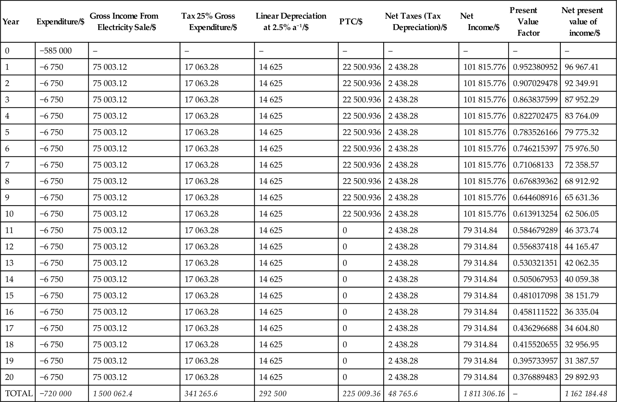
Tax payment per year=0.25×(75 003.12 − 6750)=$17 063.28.
However if we consider the effect of depreciation we can compute the net tax payment (net tax) as:
Net tax=tax payment − depreciation credit=17 063.28 − 14 625=$2438.28.
Then the net income stream for the first 10 years is:
Net income=Gross income − Expenditure − Net tax+PTC.
Net income=75 003.12 − 6750 − 2 438.28+22 500.93=$101 815.776.
Net present value of income stream at r=5% a−1 real rate of interest: $1 162 184.84.

25.16 Transmission and Grid Issues
Transmission costs are a major issue in wind energy development. Some of the best locations for generating wind energy are far distant from the consuming industrial and population centers. Some areas have a better more reliable source of wind power than others. Although half of the Unites States’ installed wind power capacity is based in Texas and California, the greatest potential for wind generation can be found in areas where there is little demand for electrical power. For instance, there exists a significant amount of wind potential in North Dakota but there are just not a lot of people or industries in North Dakota to consume the electrical power. The highest wind speeds exist in the remote and inaccessible Aleutian Islands in Alaska and necessitate an energy storage and conveyance medium such as hydrogen from water as a transportation fuel in fuel cells. A massive upgrade of the transmission lines nationwide through the national electrical power grid using high-voltage DC instead of high-voltage AC is needed to tap those distant sources [4–7].
Where water supplies are abundant along seashores or internal lakes or rivers, the electricity produced could be used for extracting hydrogen from water through the electrolysis process. Hydrogen then can become the storage medium and energy carrier of wind energy. It would be conveyed or transmitted to the energy consumption sites possibly through the existing natural gas pipeline system which covers the United States.
Another alternative is to convert hydrogen with coal into methane gas (CH4) that could be distributed through the existing natural gas distribution grid without significant modifications. Methane itself can be converted into methanol or methyl alcohol (CH3OH) as a liquid transportation fuel.
In the long term to reduce the electrical transmission losses, one can envision superconducting electrical transmission lines cooled with cryogenic hydrogen carrying simultaneously electricity and hydrogen from the wind energy production sites to the consumption sites. Such a visionary futuristic power transmission system could also provide the electrical power for a modern mass transit system using magnetically levitated (Maglev) high-speed trains transporting goods and people supplementing the current highway system in the United States.
25.17 Discussion
Wind and other renewable sources of energy are creeping toward competitiveness and weaning out from subsidies compared with traditional electricity generated from conventional fossil and nuclear power plants. It must be admitted that the electricity from wind turbines is currently more expensive than traditional generation such as from coal or natural gas. However the future scarcity would bring cost increases as rising fuel costs wage hikes and environmental requirements will affect the costs of conventionally generated electricity but not of wind energy.
If one shares the view that the fossil fuel resources are finite and depletable and that the first signs of shortage are already appearing on the horizon; then one is compelled to recognize the threat of international vicious competition for the control of the remaining supplies of fossil fuels. This makes a compelling case for wind energy.