
Practical Method to Estimate Foundation Stiffness for Design of Offshore Wind Turbines
Saleh Jalbi, Masoud Shadlou and Subhamoy Bhattacharya, University of Surrey, Guildford, United Kingdom Email: [email protected]
Abstract
Offshore wind turbine structures (OWTs) are dynamically sensitive due to their shape and form (slender column supporting a heavy rotation mass) and also due to the different forcing functions (wind, wave, and turbine loading) acting on the structures. Designers need to ensure that the first Eigen natural frequency is not close to forcing frequencies to avoid dynamic associated effects such as resonance and fatigue damage. Such damages may result in higher maintenance costs and a lower service life. Therefore, it is crucial to get the best prediction of the first natural frequency during the early stages of a project. Other design requirements include the serviceability limit state (SLS) criteria which imposes strict pile head deflection and rotation limits. These calculations require foundation stiffness and the aim of this chapter is to provide practical methods to predict the stiffness of the foundations for any ground profile (nonuniform or layered soils) through the use of standard methods. The foundation stiffness values can then be used as an input to predict the first natural frequency of OWT system as well as checking SLS requirements. An example problem is taken to show the application of the method.
Keywords
Monopiles; foundation stiffness; eigen frequency; winkler springs; p–y curves; multilayered soils; impedance functions; FEA
16.1 Introduction
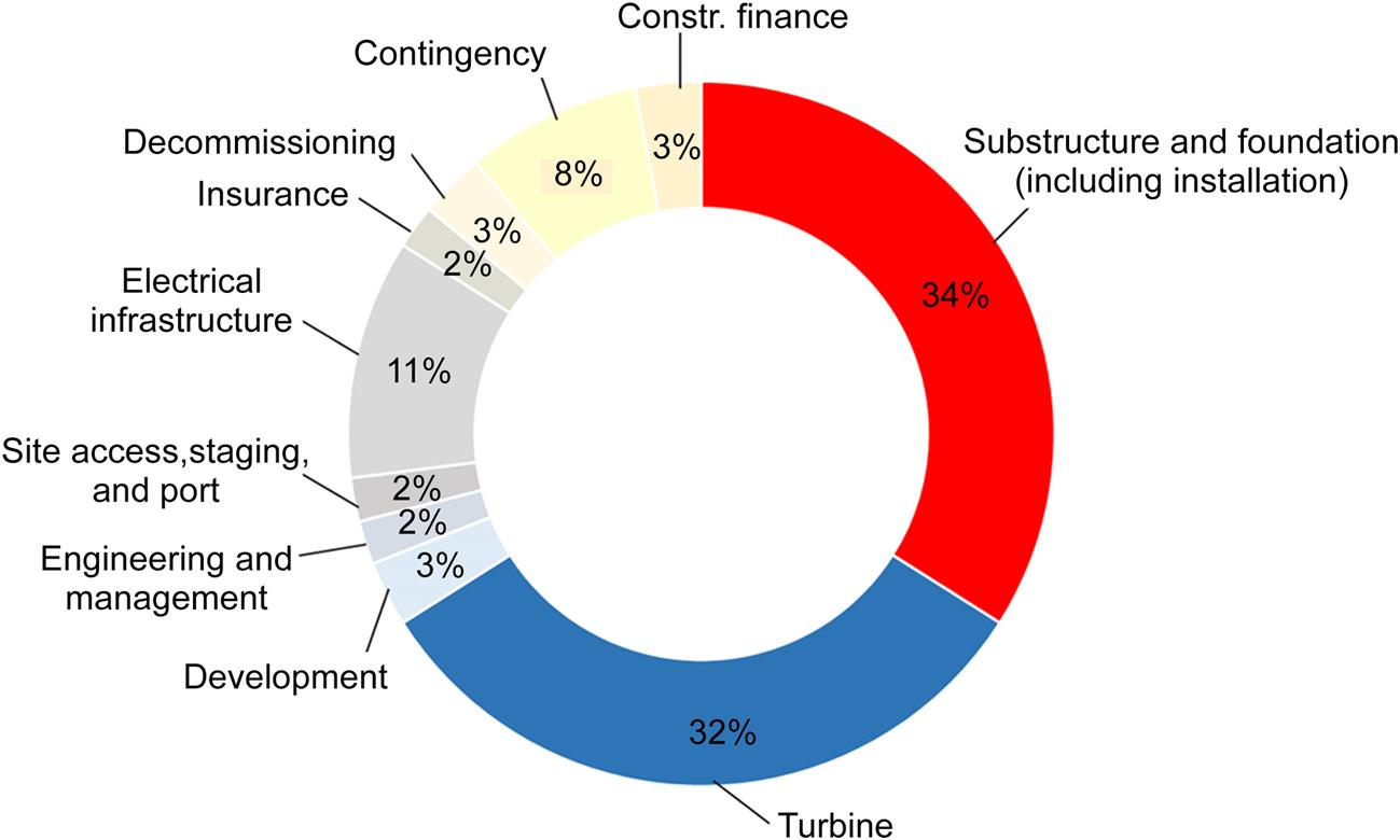
Fig. 16.1 shows a typical itemized cost of different components of an offshore wind farm and it is clear that the foundation is one of the most expensive item covering almost 34% of the overall cost. One of the main reasons of this high cost is the uncertainty associated with long-term loading conditions, ground profile, and lack of track record of performance on these structures. Research is currently under way to reduce the cost of foundations thereby reducing LCOE (levelized cost of energy). The principle aim of a foundation is to transfer all the loads from the wind turbine structure to the ground safely and within the allowable deformations. Guided by limit state design philosophy, the design considerations are to satisfy the following:
1. Ultimate limit state (ULS): This is to ensure that the maximum loads on the foundations are much lower than the capacity of the chosen foundation. This calculation is dependent on the strength of the soil.
2. Target natural frequency (Eigen frequency) and SLS: This requires the prediction of the natural frequency of the whole system (Eigen frequency) and the deformation of the foundation at the mudline level. As natural frequency is concerned with very small amplitude vibrations, linear Eigen value analysis will suffice. The deformation of the foundation will be small and prediction of initial foundation stiffness would suffice for this purpose. This requires determination of stiffness of the foundation.
3. Fatigue limit state (FLS) and long-term deformation: This would require predicting the fatigue life of the monopile as well as the effects of long-term cyclic loading on the foundation. Again this step requires stiffness of the foundation.
4. Robustness and ease of installation: This step will ascertain that the foundation can be installed and that there is adequate redundancy in the system.
Design of foundation is an iterative process and Fig. 16.2 shows a flowchart for design of monopiles suggested by Arany et al. [1]. It is clear from the flowchart that foundation stiffness plays a key role in the design. This chapter therefore focuses on the different methods of estimating the foundation stiffness and this is one of the critical parameter for design.
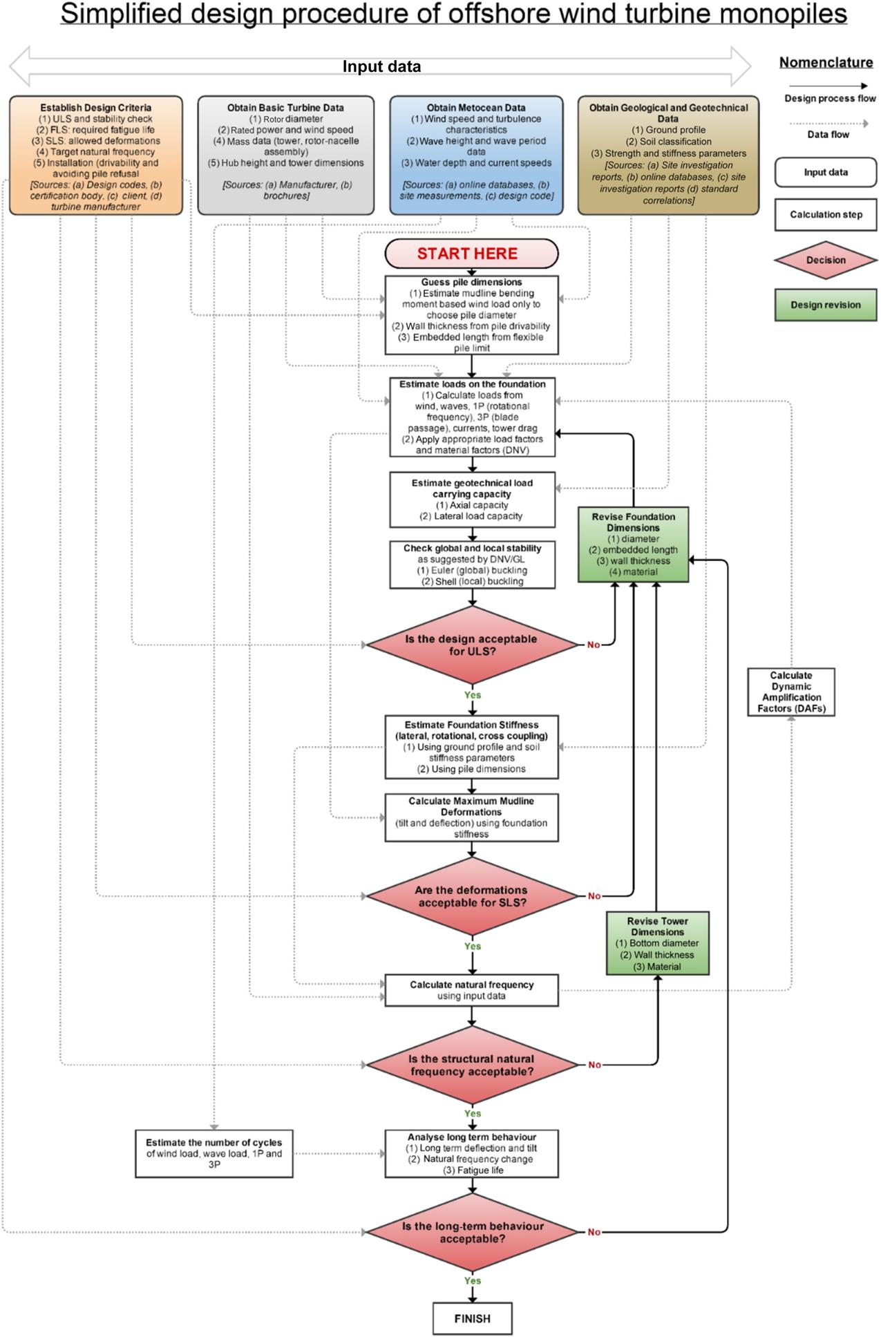
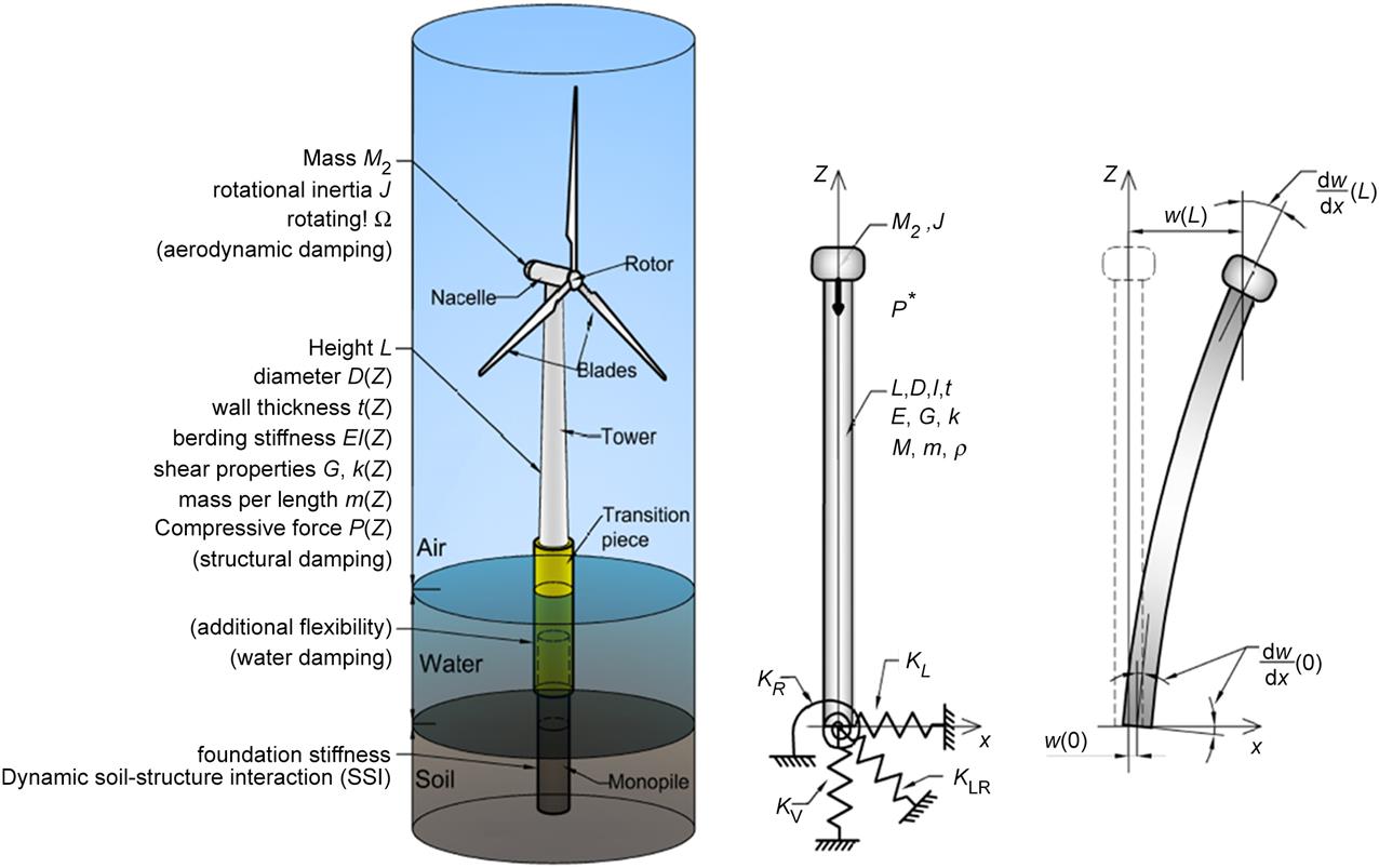
Fig. 16.3 shows a mathematical model where the foundation is replaced by a set of springs: ![]() (vertical stiffness),
(vertical stiffness), ![]() (Lateral stiffness)
(Lateral stiffness) ![]() (Rocking stiffness), and
(Rocking stiffness), and ![]() (cross-coupling). The input required to obtain
(cross-coupling). The input required to obtain ![]() ,
, ![]() and
and ![]() are: (1) pile dimensions; (2) ground profile, i.e., soil stiffness along the length of the pile. In this context, it must be mentioned that the foundation stiffness is required for two calculations: Deformation (deflection
are: (1) pile dimensions; (2) ground profile, i.e., soil stiffness along the length of the pile. In this context, it must be mentioned that the foundation stiffness is required for two calculations: Deformation (deflection ![]() and rotation
and rotation ![]() at mudline) and natural frequency estimation.
at mudline) and natural frequency estimation.
Few points may be noted regarding these springs:
1. The properties and shape of the springs (load–deformation characteristics, i.e., lateral load–deflection or moment–rotation) should be such that the deformation is acceptable under the working load scenarios expected in the lifetime of the turbine. Further details of shape of these springs associated with stress–strain of the supporting soil can be found in Bouzid et al. [2].
2. The values of the springs (stiffness of the foundation) are necessary to compute the natural period of the structure using linear Eigen value analysis. Further details on the analysis required can be found by Adhikari and Bhattacharya [3]; Adhikari and Bhattacharya [4]; Arany et al. [5]; and Arany et al. [6].
The values of the springs will also dictate the overall dynamic stability of the system due to its nonlinear nature. It must be mentioned that these springs are not only frequency dependent but also change with cycles of loading due to dynamic soil–structure interaction. Further details on the dynamic interaction can be found by Bhattacharya et al. [7]; Bhattacharya et al. [8]; Bhattacharya [9]; Lombardi et al. [10]; Zania [11]; and Damgaard et al. [12].
16.2 Methods to Estimate Foundation Stiffness
In this section three methods are discussed:
1. Simplified method: Closed-form solutions for foundation stiffness can be obtained for simple ground profiles, see Fig. 16.4. Any spreadsheet programs or even a simple calculator can be used to compute them and typically time take is only few minutes. This method can be useful in the preliminary design and during the optimization stage or even financial feasibility study. In this context it must be remembered that foundation constitutes 34% of the overall cost.
2. Standard method: This is one of the most common methods used in industry, see Fig. 16.5. Foundation–soil interaction is represented by a set of discrete Winkler springs where the spring stiffness is obtained through p–y curves which are provided in different design standards. Standard software are available at reasonable costs to carry the analysis and will only take few hours to carry out an analysis. Complex ground soil profiles can be analyzed for standard soils, i.e., sand and clay. Few soil parameters are required and the effects of cyclic load are taken empirically.
3. Advanced methods: These are continuum models (Fig. 16.6) and advanced 3D finite element software packages or programs are necessary. Such packages are expensive, computationally demanding, and require experienced engineer to run the simulations. These models are versatile and can model complex ground profile and any type of soils. Cyclic loading can also be applied.


16.2.1 Simplified Method (Closed-Form Solutions)
Closed-form solutions have been proposed by Shadlou and Bhattacharya [13]. Values of ![]() ,
, ![]() and
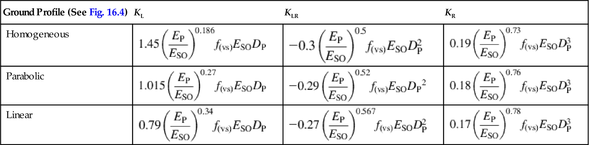
and ![]() are summarized in Tables 16.1 and 16.2 for rigid and flexible piles for three types of ground profile: homogenous, linear, and parabolic, see Fig. 16.4. Homogeneous soils are soils which have a constant stiffness with depth such as over-consolidated clays. On the other hand, a linear profile in typical for normally consolidated clays and parabolic behavior can be used for sandy soils. It may be observed from Table 16.1 that the stiffness term is a function of the aspect ratio (L/Dp) of the pile and soil stiffness (ES0) and this is a characteristic of rigid behavior. Table 16.2 is a function of relative pile–soil stiffness (EP/ES). Further details of classification of rigid and flexible piles in relation to monopile application can be found by Shadlou and Bhattacharya [13].
are summarized in Tables 16.1 and 16.2 for rigid and flexible piles for three types of ground profile: homogenous, linear, and parabolic, see Fig. 16.4. Homogeneous soils are soils which have a constant stiffness with depth such as over-consolidated clays. On the other hand, a linear profile in typical for normally consolidated clays and parabolic behavior can be used for sandy soils. It may be observed from Table 16.1 that the stiffness term is a function of the aspect ratio (L/Dp) of the pile and soil stiffness (ES0) and this is a characteristic of rigid behavior. Table 16.2 is a function of relative pile–soil stiffness (EP/ES). Further details of classification of rigid and flexible piles in relation to monopile application can be found by Shadlou and Bhattacharya [13].
Table 16.1
Formulas for Stiffness of Monopiles Exhibiting Rigid Behavior
| Ground Profile (See Fig. 16.4) | KL | KLR | KR |
| Homogeneous | |||
| Parabolic | |||
| Linear |
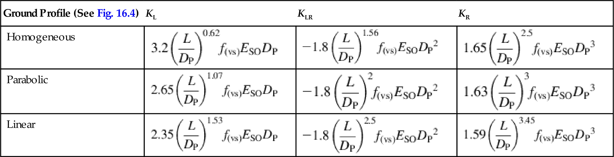
Table 16.2
Tables for Monopiles Exhibiting Flexible Behavior
| Ground Profile (See Fig. 16.4) | KL | KLR | KR |
| Homogeneous | |||
| Parabolic | |||
| Linear |
16.2.2 Standard Method
Traditionally in the offshore industry, a nonlinear p–y method is employed to find out pile head deformations (deflection and rotation) and foundation stiffness. The approach can be found in API [14] and also suggested in DNV [15]. Originally it was developed by Matlock [16]; Reese et al. [17]; O’Neill and Murchinson [18], and the basis of this methodology is the Winkler approach [2] whereby the soil is modeled as independent springs along the length of the pile, see Fig. 16.5. The p–y approach uses nonlinear springs and produces reliable results for cases in which it was developed, i.e., small diameter piles and for few cycles of loading. The method is not validated for large diameter piles, in fact, using this method, underprediction of foundation stiffness has been reported by Kallehave and Thilsted [19], who also proposed an updated p–y formulation. Many researchers have recently worked on developing design methodologies for the large diameter more stocky monopiles with length to diameter ratios typically in the range between 4 and 10.
16.2.3 Advanced Method
In this method, soil–structure interaction is carried out using 2D and 3D FEA (finite element analysis) and different sophisticated soils models can be used. This requires advanced soil testing to feed the soil parameters. It is important to note that such models usually require not only knowledge but also expertise and experience. It is not advisable to use this method during the preliminary and optimization stages due to the high cost and the time required for calculation. This method best serves as a final check to a few optimized cases as results obtained are usually of high accuracy. Fig. 16.6 shows a typical section through a finite element model with various degrees of freedom showing the soil mass, the pile, the pile–soil interface, and the boundary conditions.
16.3 Obtaining Foundation Stiffness From Standard and Advanced Method
The analysis method presented in Sections 16.2.2 and 16.2.3 are numerical methods and the output from such analysis will be pile head load–deflection and moment–rotation curves. However, following Fig. 16.3, three stiffness terms (KL, KR, and KLR) are required to carry out dynamic and SLS calculations. This section of the chapter explains a simple methodology to extract the stiffness terms from the analysis results obtained in Sections 16.2.2 and 16.2.3.
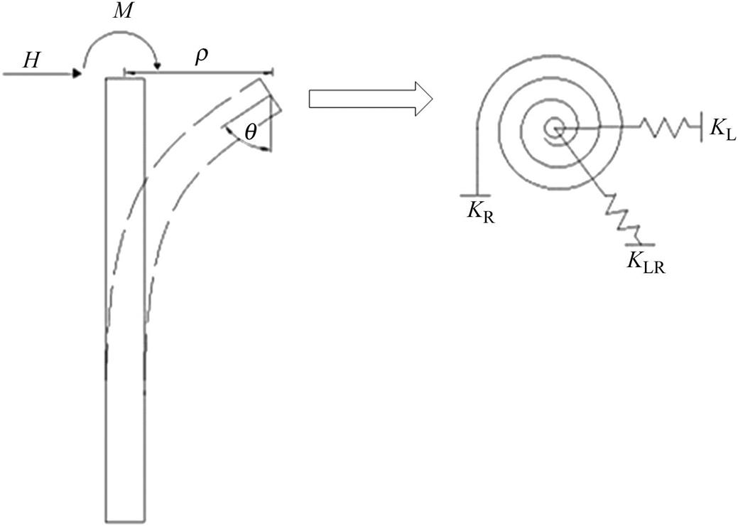
While KL (lateral stiffness, i.e., force required for unit lateral deflection and the unit is MN m−1) and KR (rocking stiffness is the moment required for unit rotation and the unit is MNm rad−1) are easy to appreciate and visualize, the cross-coupling term (KLR) is more involved and arises from matrix compliance. Arany et al. [5] showed cross-coupling stiffness (KLR) of the foundation is an important parameter and must be considered for dynamic analysis of monopiles. Gazetas [20] explains the coupling effect in foundations as a consequence of the inertia of the structure and where the foundation center of gravity is above the center of soil reaction pressure. This means as the structure is being displaced laterally, an inertial force arises at the center of gravity and produces a net moment thereby rocking occurs. It is therefore necessary to explain the cross-coupling term (KLR) through a simple cantilever beam example as shown in Fig. 16.7.
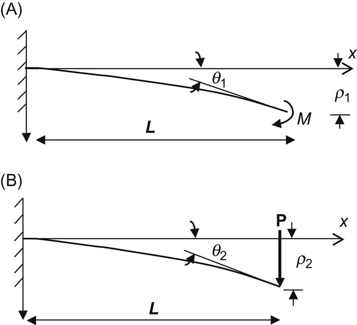
Fig. 16.7A shows a cantilever beam subjected to a moment at the free end (M) causing deflection (ρ1) and rotation (θ1). On the other hand, Fig. 16.7B shows another cantilever beam where the lateral load (P) at the tip causes deflection (ρ2) and rotation (θ2). The expressions for deflection and rotation are given by Eqs. (16.1) and (16.2).
(16.1)
For a point load
(16.2)
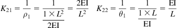
It is clear that both the moment and the point load produce a rotation as well as a deflection and in effect the rotation caused by the point load or the deflection caused by the moment is indicative of the cross-coupling stiffness term. By definition, the stiffness is the force/moment required to move the body by a unit displacement/rotation respectively, and thus for this example K11 is the stiffness resisting the point load, K12 and K21 are cross-coupling stiffness, and K22 is the stiffness resisting rotation. For “unit” values for P and M, the stiffness terms are given by Eqs. (16.3) and (16.4).
(16.3)
 (16.3)
(16.4)
 (16.4)
It may be noted that the cross-coupling stiffnesses K12 and K21 are equal for the same magnitude of loading. This method can be extended to the results obtained from standard and advanced methods to find the three stiffness terms (KL, KLR, and KR). Typically (pile head load)–deflection and (pile head moment)–rotation curves are nonlinear depending on the soil type. However, the linear range of the curves can be used to estimate pile head rotation and deflection based on Eq. (16.5) and one can understand the importance of cross-coupling term.
(16.5)
Eq. (16.5) can be rewritten as Eq. (16.6) through matrix operation where I (impedance matrix) is a 2×2 matrix given by Eq. (16.7).
(16.6)
(16.7)
To obtain the stiffness terms, a numerical model (either standard or advanced) could be analyzed for a lateral load (say H=H1) with zero moment (M=0) and obtain values of deflection and rotation (ρ1 and θ1). The results can be expressed through Eqs. (16.8) and (16.9).
(16.8)
(16.9)
Similarly another numerical analysis can be done for a defined moment (M=M1) and zero lateral load (H=0) results are shown in Eqs. (16.10) and (16.11).
(16.10)
(16.11)
From the above analysis (Eqs. (16.8)– (16.11)), terms for the I matrix (Eq. (16.7)) can be obtained. Eq. (16.6) can be rewritten as Eq. (16.12) through matrix operation.
(16.12)
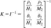
Comparing Eqs. (16.5) and (16.12), it can be observed that the relation between the stiffness matrix and the inverse of impedance matrix (I) given by Eq. (16.13). Eqs. (16.14) and (16.15) are matrix operations which can be carried out easily to obtain KL, KR, and KLR.
(16.13)
(16.14)
 (16.14)
(16.15)
 (16.15)
Therefore, mathematically, it is required to run only two cases, i.e., p–y analyses or FEA to obtain the three spring stiffness. It is important to note that the above methodology is only applicable in the linear range and therefore it is advisable to obtain a load–deflection and moment–rotation curve to check the range of linearity. If the analysis is used beyond the linear range, underestimations of deflections and rotations will occur. Also the natural frequency of the whole system will be underestimated.
16.3.1 Example Problem (Monopile for Horns Rev 1)
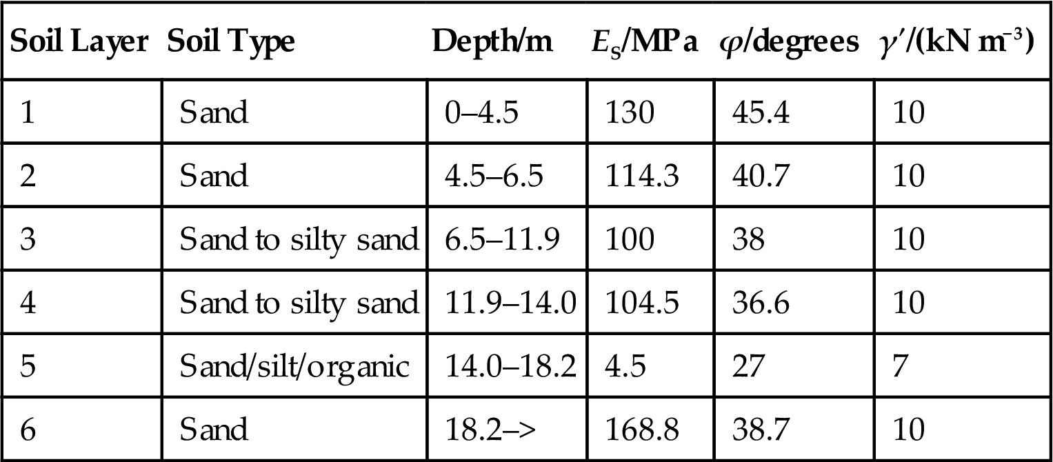
The case study of Horns Rev 1 is used to show the application of the methodology. Various data on the case study can be found by Augustensen et al. [20]. The monopile foundation supports a 60 m long tower carrying a Vestas V80 2 MW wind turbine. The pile has a diameter of 4.0 m and varying wall thickness (WT in Fig. 16.8). The reported ultimate loads on the pile head were H=4.6 MN and M=95 MN.m. Table 16.3 provides a detailed description of the soil layers which was obtained through an extensive test program including geotechnical borings, cone penetration tests (CPTs), and triaxial tests given by Augustensen et al. [21]. ALP (Oasys) has been used for the p–y analysis of the monopile which can compute deflections, rotations, and bending moments along the pile. Several other software packages such as PYGM and LPILE are available for this type of analysis, or can be solved numerically through a MATLAB program. In this study, p–y curves along different depths are modeled in two ways: (1) elastic–plastic springs by taking the soil properties given in Table 16.3; (2) API recommended p–y springs.
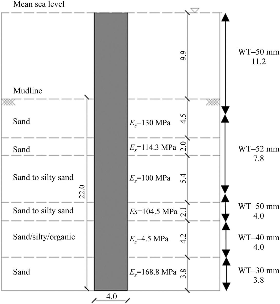
Table 16.3
| Soil Layer | Soil Type | Depth/m | ES/MPa | ϕ/degrees | γ′/(kN m−3) |
| 1 | Sand | 0–4.5 | 130 | 45.4 | 10 |
| 2 | Sand | 4.5–6.5 | 114.3 | 40.7 | 10 |
| 3 | Sand to silty sand | 6.5–11.9 | 100 | 38 | 10 |
| 4 | Sand to silty sand | 11.9–14.0 | 104.5 | 36.6 | 10 |
| 5 | Sand/silt/organic | 14.0–18.2 | 4.5 | 27 | 7 |
| 6 | Sand | 18.2–> | 168.8 | 38.7 | 10 |
The API code provides the following formulations for sandy soils:
(16.16)
where A is a factor that depends on the type of loading and pu depends on the depth and angle of internal friction ϕ′.
However for the elastic–plastic model used in the study, the following equations were used to construct the p–y curves.
(16.17)
where h is the midpoint of the elements immediately above and below the spring under consideration.
The plastic phase of the curve is given by:
(16.18)
where Kq and Kc are factors that depend on depth and ϕ′ [22].
Fig. 16.9 shows the results obtained from the analysis.
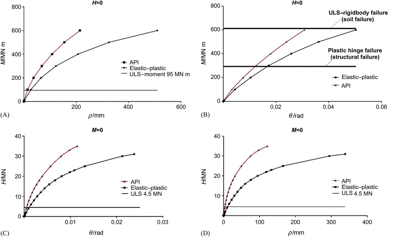
It is evident from the Fig. 16.9 that the ULS loads lie within the linear range which means the deflections and rotations arising from such forces can be estimated using KL, KR, and KLR. Table 16.4 summarizes the results for the analysis where two load cases have been applied (H=0.2 MN and M=0), and (H=0 and M=0.2 MN m) where the major steps are also shown. It may also be noted that Fig. 16.9B plots the ultimate capacity of the pile based on two considerations: (1) soil fails and the pile fails as rigid body failure and (2) pile fails by forming plastic hinge.
Table 16.4
Results from Analysis and Computation of I Matrix
| Model | Loads | ρ/mm | θ/rad | IL/(m/MN) | ILR/(rads/MN) | IRL/(m/MN.m) | IR/(rads/MN.m) |
| Elastic–plastic | H=0.2 MN m | 0.43 | 4.1E−05 | 2.15E−03 | 2.1E−04 | 0 | 0 |
| M=0 MN m | |||||||
| API code | H=0.2 MN m | 0.15 | 2.3E−05 | 7.5E-04 | 1.1E−04 | 0 | 0 |
| M=0 MN m | |||||||
| Elastic–plastic | M=2 MN m | 0.41 | 8.3E−05 | 0 | 0 | 2.1E−04 | 4.2E−05 |
| H=0 MN | |||||||
| API code | M=2 MN m | 0.223 | 6.0E−05 | 0 | 0 | 1.1E−04 | 3.0E−05 |
| H=0 MN m |

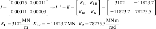
Using Eq. (16.13) and applying to the results obtained and shown in Table 16.4, stiffness terms as predicted by elastic–plastic model is given in Eq. (16.19).
Elastic–plastic formulation
(16.19)
 (16.19)
The same approach has been used for the API model and the results are shown in Eq. (16.20).
API formulation
(16.20)
 (16.20)
It may be noted that the stiffness terms are quite different in the two formulations given in Eqs. (16.19) and (16.20). This is because the API formulation is empirical and is calibrated against small diameter piles and the extrapolation to large diameter piles is not validated or verified.
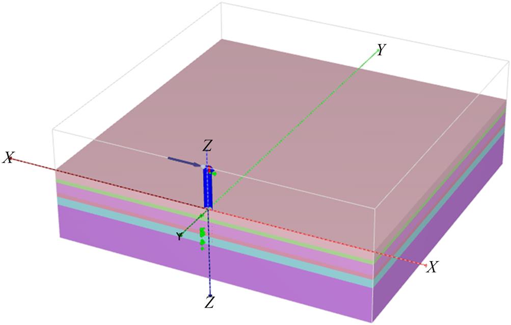
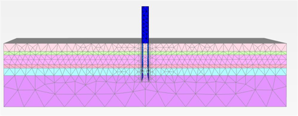
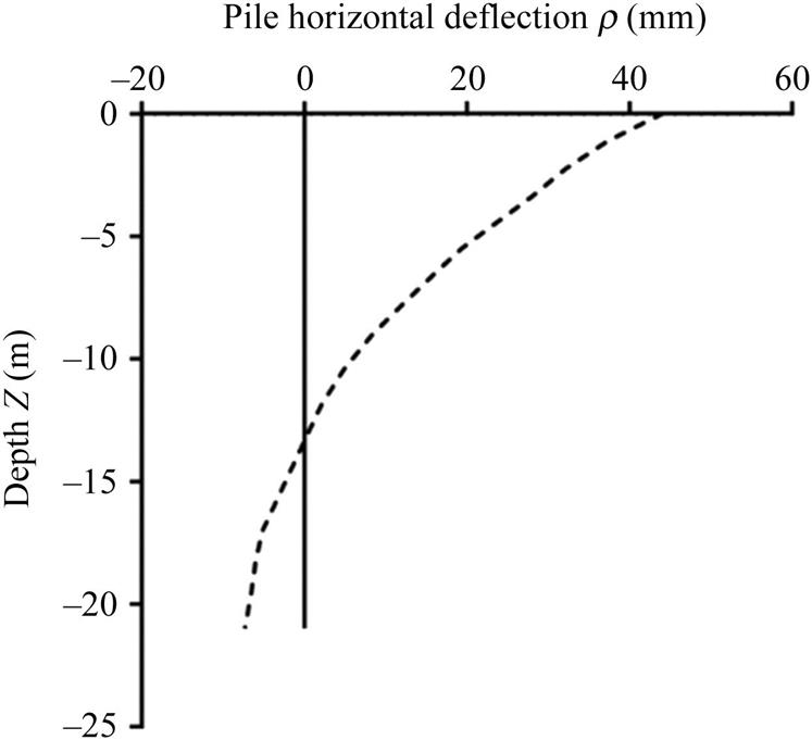
Finite element software package PLAXIS 3D was also used to evaluate the deflection and rotation due to the pile head loads. To save computational efforts space, half the pile was modeled (Figs. 16.10 and 16.11). A classical Mohr–Coulomb material model was set for the soil with the same stiffness and strength properties provided in Table 16.3. For the pile material, elastic perfectly plastic model was used. Ten node tetrahedral elements were assigned to the soil volume and six node triangular plate elements were used for the pile. The interface between the soil and the pile was modeled with double noded elements. The soil extents were set as 20Dp, and a medium fine mesh was used. The pile was extended by 21 m above the ground to simulate the effect of the applied moment. Similar plots such as that shown in Fig. 16.9 were obtained. Fig. 16.12 plots the deflection along the length of the pile obtained for H=4.6 MN and M=95 MN m.
16.4 Discussion and Application of Foundation Stiffness
Fig. 16.13 schematically shows the essence of the matrix operations presented in the earlier section. Essentially, the foundation is replaced by a set of springs which are obtained from lateral load/moment analysis of piles. This is quite similar to substructure method.
16.4.1 Pile Head Deflections and Rotations
Eq. (16.5) can be used to predict pile head deflections and rotations as shown in Eq. (16.21). It may be noted from Fig. 16.9 that the ultimate loads were within the linear range.
(16.21)
 (16.21)
The results predict a deflection of 30 mm and a rotation of 0.280° (degree) using elastic–plastic model. On the other hand, the results predict 14 mm of deflection and 0.20° using API model. The advanced model based on PLAXIS 3D shown in Fig. 16.12 predicts a deflection of 42.5 mm and a rotation of 0.3°.
16.4.2 Prediction of the Natural Frequency
These foundation stiffness values can be used to predict natural frequency following the method proposed by Arany et al. [1]. The steps are also shown as follows.
Step 1: Fixed based natural frequency of the tower
Calculate the bending stiffness ratio of tower to the pile:
(16.22)
Calculate the platform/tower length ratio:
(16.23)
Calculate the substructure flexibility coefficient to account for the enhanced stiffness of the transition piece:
(16.24)
 (16.24)
Obtain the fixed base natural frequency of the tower:
(16.25)
 (16.25)
where the cross-sectional properties of the tower can be calculated as:
(16.26)
Step 2: Calculate the nondimensional foundation stiffness parameters
The equivalent bending stiffness of tower needed for this step:
(16.27)
where Itop is the second moment of area of the top section of the tower.
(16.28)
(16.29)
(16.30)
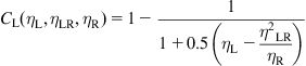
Step 3: Calculate the foundation flexibility factors
(16.31)
 (16.31)
16.32)
 16.32)
Step 4: Calculate the flexible natural frequency of the offshore wind turbine structure (OWT) system
(16.33)
Due to lack of the some aspects of tower data, a similar 2 MW wind turbine from North Hoyle has been used. Table 16.5 summarizes the tower properties used for the calculations.
Table 16.5
| Top diameter/m | 2.3 |
| Bottom diameter/m | 4.0 |
| Wall thickness/mm | 35 |
| Tower height/m | 70 |
| Mass of RNA/t | 100 |
| Mass of tower/t | 130 |
For simplicity the substructure flexibility coefficient (CMP) is considered to be 1. Therefore, following Eqs. (16.22)– (16.33), we obtain:
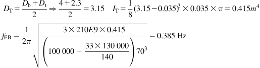
The fixed base frequency is therefore 0.385 Hz.

The nondimensional groups are:
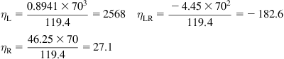
The foundation flexibility coefficients are given as follows:
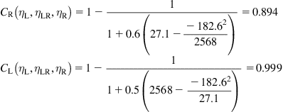
The natural frequency is therefore given by:
16.4.3 Comparison With SAP 2000 Analysis
The system was modeled using SAP 2000 and a modal analysis is carried out to obtain the natural frequency. Nonprismatic beam elements of varying diameter were assigned to the tower while the soil–structure interaction was represented by discrete linear Winkler springs. The spring stiffness values were taken from the soil properties (Table 16.3) and are a function of modulus of elasticity at the location of the spring and the spacing between two adjacent springs. A lumped mass was assigned at the tower head to model the dead mass of the RNA (rotor nacelle assembly). The first natural frequency recorded was 0.351 Hz and Fig. 16.14 shows the first mode of vibration.

Nomenclature
CL, CR Lateral and rotational flexibility coefficient
CMP Substructure flexibility coefficient
ES Vertical distribution of soil’s Young’s modulus
ESO Initial soil Young’s modulus at 1Dp depth
EIη Equivalent bending stiffness for tower top loading
f0 First natural frequency (flexible)
fFB Fixed base (cantilever) natural frequency
H Horizontal load at pile head
IT Tower second moment of area
KL Lateral stiffness of the foundation
KLR Cross-coupling stiffness of the foundation
KR Rotational stiffness of the foundation
M Applied moment at the pile head
mRNA Mass of rotor nacelle assembly
ηL Nondimensional lateral stiffness
ηLR Nondimensional cross-coupling stiffness