
Physical Modeling of Offshore Wind Turbine Model for Prediction of Prototype Response
Domenico Lombardi1, Subhamoy Bhattacharya2 and George Nikitas2, 1The University of Manchester, Manchester, United Kingdom, 2University of Surrey, Guildford, United Kingdom Email: 1[email protected]
Abstract
Offshore wind turbines (OWTs) are considered as an important element of the future energy infrastructure. The majority of operational OWTs are founded on monopiles in water depths up to 30 m. Alternative foundation arrangements, however, are needed for future development rounds in deeper waters. To date, there have been no long-term observations of the performance of these relatively novel structures, although the monitoring of a limited number of OWTs has indicated a departure of the system dynamics from the design requirements. Lack of data concerning long-term performance indicates a need for detailed investigation to predict the future performance of such structures. Arguably this can be best carried out through small-scale laboratory experimental investigation, whose results are interpreted based on appropriate scaling laws. In this chapter, scaling laws are derived for the design of such model tests, which can be used for studying the long-term performance of small-scale wind turbines and prediction of the prototype response.
Keywords
Physical modeling; dimensional analysis; dynamics; resonance; long-term behavior; soil–structure interaction
17.1 Introduction
OWTs are providing an increasing proportion of wind energy generation capacity because offshore sites are characterized by stronger and more stable wind conditions than comparable onshore sites. Owing to the higher capacity factor (i.e., ratio of the actual amount of power produced over a period of time to the rated turbine power) and decreasing levelized cost of energy (LCOE) (i.e., ratio of the total cost of an offshore wind farm to the total amount of electricity expected to be generated over the wind farm’s lifetime), offshore wind turbines (OWTs) are currently installed in high numbers in Northern Europe. The industry is rapidly developing worldwide, particularly in countries such as China, South Korea, Taiwan, and Japan, whereas the United States has recently installed its first pilot offshore wind farm in Block Island. The design and construction of offshore turbines, however, are more challenging when compared with onshore counterparts, owing to the harsh environmental conditions existing at the offshore sites.
17.1.1 Complexity of External Loading Conditions
OWTs are characterized by a unique set of dynamic loading conditions that is schematically depicted in Fig. 17.1. These include: (1) load produced by the turbulence in the wind, whose amplitude is function of the wind speed; (2) load caused by waves crashing against the substructure, whose magnitude depends on the height and period of waves; (3) load caused by mass and aerodynamic imbalances of the rotor, whose forcing frequency equals the rotational frequency of the rotor (referred to as 1P loading in the literature); (4) loads in the tower due to the vibrations caused by blade shadowing effect (referred to as 3P loading in the literature), which occurs as each blade passes through the shadow of the tower.
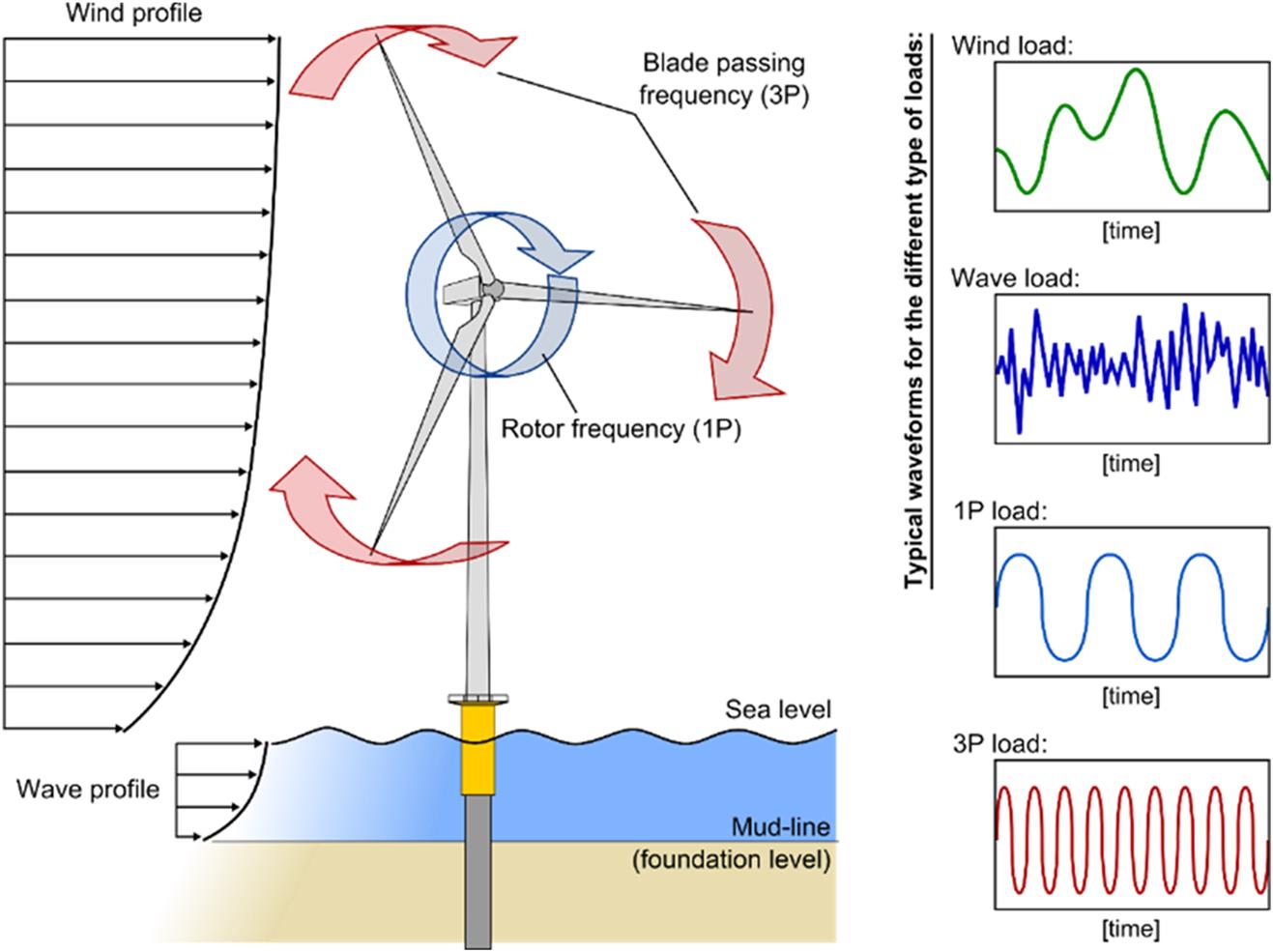
The loads imposed by wind and wave are random in both space and time, as a result these are better described statistically by using the Pierson–Moskowitz wave spectrum and Kaimal wind spectrum, as shown in Fig. 17.2. It is clear from the frequency content of the applied loads that the designer in order to avoid the resonance of the OWT has to select a design frequency that lies outside the ranges of forcing frequencies. Specifically, the Det Norske Veritas (DNV) code [1] recommends that the natural frequency of the wind turbine should be at least ±10% away from the main forcing frequencies introduced earlier. Depending on the design value of natural frequency, three design approaches are possible, namely, soft–soft (natural frequency <1P), soft–stiff (natural frequency between 1P and 3 P), and stiff–stiff (natural frequency >3P).

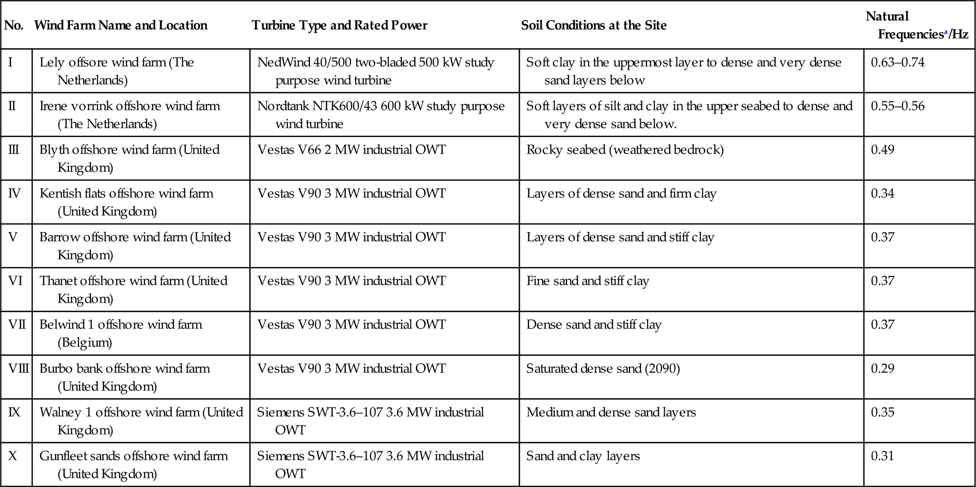
It is worth noting that the design procedure requires an accurate evaluation of the natural frequency, which is dependent on the support condition (i.e., the stiffness of the foundation) that in turn relies on the strength and stiffness of the surrounding soil. Furthermore, as the natural frequencies of OWTs are very close to the forcing frequencies, the dynamics pose multiple design challenges because of the tight tolerance of the target natural frequency, whereby the scale of the challenges will vary depending on turbine types and site characteristics. Typical values of vibration characteristics and site characteristics of operating wind turbines are listed in Table 17.1.
Table 17.1
Analyzed Offshore Wind Farms With the Used Wind Turbines and Soil Conditions at the Sites
| No. | Wind Farm Name and Location | Turbine Type and Rated Power | Soil Conditions at the Site | Natural Frequenciesa/Hz |
| I | Lely offsore wind farm (The Netherlands) | NedWind 40/500 two-bladed 500 kW study purpose wind turbine | Soft clay in the uppermost layer to dense and very dense sand layers below | 0.63–0.74 |
| II | Irene vorrink offshore wind farm (The Netherlands) | Nordtank NTK600/43 600 kW study purpose wind turbine | Soft layers of silt and clay in the upper seabed to dense and very dense sand below. | 0.55–0.56 |
| III | Blyth offshore wind farm (United Kingdom) | Vestas V66 2 MW industrial OWT | Rocky seabed (weathered bedrock) | 0.49 |
| IV | Kentish flats offshore wind farm (United Kingdom) | Vestas V90 3 MW industrial OWT | Layers of dense sand and firm clay | 0.34 |
| V | Barrow offshore wind farm (United Kingdom) | Vestas V90 3 MW industrial OWT | Layers of dense sand and stiff clay | 0.37 |
| VI | Thanet offshore wind farm (United Kingdom) | Vestas V90 3 MW industrial OWT | Fine sand and stiff clay | 0.37 |
| VII | Belwind 1 offshore wind farm (Belgium) | Vestas V90 3 MW industrial OWT | Dense sand and stiff clay | 0.37 |
| VIII | Burbo bank offshore wind farm (United Kingdom) | Vestas V90 3 MW industrial OWT | Saturated dense sand (2090) | 0.29 |
| IX | Walney 1 offshore wind farm (United Kingdom) | Siemens SWT-3.6–107 3.6 MW industrial OWT | Medium and dense sand layers | 0.35 |
| X | Gunfleet sands offshore wind farm (United Kingdom) | Siemens SWT-3.6–107 3.6 MW industrial OWT | Sand and clay layers | 0.31 |
aEstimated based on Arany L, Bhattacharya S, Macdonald JH, Hogan SJ. Closed form solution of Eigen frequency of monopile supported offshore wind turbines in deeper waters incorporating stiffness of substructure and SSI. Soil Dyn Earthq Eng 2016;83:18–32 [16].
17.1.2 Design Challenges
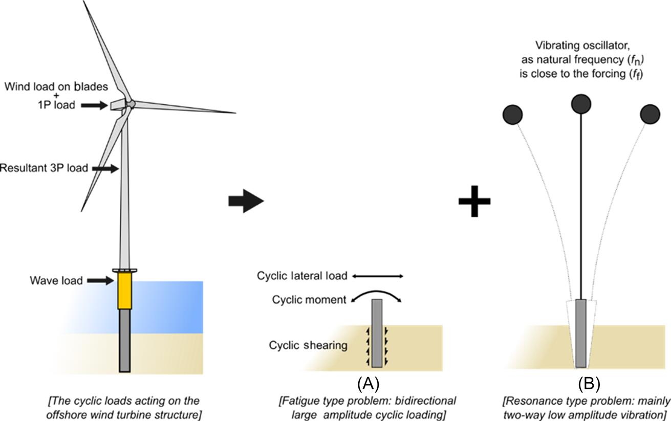
There are two main aspects related to cyclic loading conditions, see Nikitas et al. [2], that have to be taken into account during design: (1) soil behavior due to nondynamic repeated loading, i.e., fatigue-type problem and this is mainly attributable to wind loading which has a very low frequency; (2) soil behavior due to dynamic loading which will cause dynamic amplification of the foundation response, i.e., the resonance-type problem. This is due mainly due to 1P and 3P loading but wave loading can also be dynamic for deeper waters and heavier turbines. A breakdown of the overall problem of soil–structure interaction into two types of soil shearing is schematically represented in Fig. 17.3. The current codes of practice (e.g., DNV [1], American Petroleum Institute, API [2,3], Institute of Electrical Engineers, IEC [4]) for the design of monopile foundations of OWTs recommend the application of the p–y curves primarily for the evaluation of lateral pile capacity in the ultimate limit state. The codes provide limited guidance in predicting the change of the foundation stiffness and consequent change of natural frequency, which are both design drivers for serviceability limit state requirements.
Furthermore, it is important to note that the vibration of the foundation will induce cyclic strains in the soil in its vicinity. Under moderate-to-high amplitudes of cyclic loading, most soils change their stiffness and strength. In order to study the changes in soil stiffness due to these cyclic strains, the developing strain in the soil around the shear zone must be taken into consideration. Soils in offshore sites can be fully saturated and therefore pore pressures are likely to develop as a result of these cyclic strains. The pore pressure developed may dissipate to the surrounding soil depending on factors including frequency of loading, permeability of the soil, and diameter of the pile. Pore water pressure may also develop in unsaturated soils under cyclic shearing. It should be noted that due to the nature of the external excitation, wave and wind-induced loads may impose either one-way or two-way cyclic loading on the monopile, whereby one-way loading develops more soil deformation and consequently more change in foundation stiffness.
OWTs are relatively new structures without any track record of long-term performance. Therefore, the uncertainties of their long-term response pose additional challenges to developers and designers of offshore wind farms. In fact, monitoring of a limited number of installed wind turbines has indicated a gradual departure of the overall system dynamics from the design requirements (e.g., the data from Lely wind farm data [5]), which may lead to amplification of the dynamic response of the turbines, leading to larger tower deflections and/or rotations beyond the allowable limits tolerated by manufacturer. The latter are often considered responsible for the damage observed in gearboxes and other electrical-rotating equipment.
17.1.3 Technical Review/Appraisal of New Types of Foundations
Foundations typically cost 25%–35% of an overall offshore wind farm project and in order to reduce the LCOE, new innovative foundations are being proposed. However, before any new type of foundation can actually be used in a project, a thorough technology review is often carried out to de-risk it. European Commission defines this through TRL (Technology Readiness Level) numbering starting from 1 to 9; see Table 17.2 for different stages of the process. One of the early works that needs to be carried out is technology validation in the laboratory environment (TRL-4). In this context of foundations, it would mean carrying out tests to verify the long-term performance. It must be realized that it is very expensive and operationally challenging to validate in a relevant environment and therefore laboratory-based evaluation has to be robust so as to justify the next stages of investment. This is another motivation for scaled model testing.
Table 17.2
TRL Level as European Commission
TRL-1: Basic principles verified
TRL-2: Technology concept formulated
TRL-3: Experimental proof of concept
TRL-4: Technology validated in laboratory
TRL-5 Technology validated in relevant environment
TRL-6: Technology demonstrated in relevant environment
TRL-7: System prototype demonstration in operational environment
TRL-8: System complete and qualified
TRL-9: Actual system proven in operational environment
17.1.4 Physical Modeling for Prediction of Prototype Response
Experimental investigations on physical wind turbine models can provide valuable information for understanding the dynamic behavior and long-term performance of OWTs. While physical modeling at normal gravity (often known as 1 g testing) can be used for modeling different loading conditions experienced by structures, its application in tackling soil–structure interaction needs additional consideration. In such cases, geotechnical centrifuge facilities are often used where 1:N scale model can be subjected to N g (N times earth gravity) to replicate the prototype stresses. However, OWTs are very complex structure involving aerodynamics (wind turbulence at the blades), hydrodynamics (wave slamming the tower and the part of the tower under water), cyclic, and dynamic soil–structure interaction. Ideally, a wind tunnel and a wave tank onboard a geotechnical centrifuge is suitable which seems to be unlikely with the current technology development. For such problems involving many interactions, where overall system dynamics and long-term performance needs to be studied, centrifuge is not well suited due to the unwanted parasitic vibration of geotechnical centrifuge and the lack of stable platform. Another important limitation of centrifuge facilities is the limited number of cycles that can reasonably be applied when compared with the expected number of cycles that a typical OWT experiences over its life span of 25 years, which is in the range 107–108. This calls for alternative modeling techniques where a problem will be studied through a set of nondimensional groups and is explained in the next section.
17.2 Physical Modeling of OWTs
Derivation of correct scaling laws constitutes the first step in an experimental study. The similitude relationships are essential for interpretation of the experimental data and for scaling up the results for the prediction of the prototypes’ responses. As shown in Fig. 17.4, there are two approaches for deriving the scaling law relationships. The first is to use standard tables for scaling and multiply the model observations by the scale factor to predict the prototype response, see for example Wood [6]. The alternative is to study the underlying mechanics/physics of the problem based on the model tests, recognizing that not all the interactions can be scaled accurately in a particular test. Once the mechanics/physics of the problem are understood, the prototype response can be predicted through analytical and/or numerical modeling in which the physics/mechanics discovered will be implemented in a suitable way. As shown by Bhattacharya et al. [7] and Lombardi et al. [8], the second method is well suited for investigating the dynamics of OWTs, which involves complex dynamic wind–wave–foundation–structure interaction and no physical modeling technique can simultaneously satisfy all the interactions at a single scale. Ideally, a wind tunnel combined with a wave tank on a geotechnical centrifuge would serve the purpose but this is unfortunately not feasible. Special consideration is required when interpreting the test results.

The design and interpretation of test carried out on a small-scale model require the assessment of a set of laws of similitude that relate the model to the prototype structure. These can be derived from dimensional analysis from the assumptions that every physical process can be expressed in terms of nondimensional groups and the fundamental aspects of physics must be preserved in the design of model tests. The necessary steps associated with designing such a model can be stated as follows:
• To deduce the relevant nondimensional groups by thinking of the mechanisms that govern the particular behavior of interest at both model and prototype scale.
• To ensure that a set of crucial scaling laws are simultaneously conserved between model and prototype through pertinent similitude relationships.
• To identify scaling laws which are approximately satisfied, and those which are violated and which therefore require special consideration.
17.2.1 Dimensional Analysis
Dimensional analysis refers to a method of great generality and mathematical simplicity that can be conveniently used for studying phenomena that at first appear to be very complex but which can be qualitatively analyzed and described in more simplified terms [9]. Although the basis of dimensional analysis was set in the 19th century by Fourier in his work on the theory of the heat flow, only in the 20th century the method has been extensively used in different fields of physics and engineering. The approach is based on the concept of similarity, which in physical terms implies that that any phenomenon can be studied through a finite number of independent quantities expressed in a nondimensional form, i.e., unit-free. In this context, the aim of dimensional analysis is to determine these nondimensional quantities, which constitutes the first step in an experimental study.
17.2.2 Definition of Scaling Laws for Investigating OWTs
As discussed earlier, OWTs are dynamically sensitive structures because of the multiple frequencies that contribute to the complexity of the interaction of the foundation with the supporting soil. To study the dynamics and predict the long-term performance of OWTs, the following phenomena have to be considered and correctly replicated in the model tests, namely:
• Vibration of the pile owing to the environmental loads will induce cyclic strains in the soil in the vicinity of the pile. In order to study the changes in soil stiffness owing to these cyclic strains, the developing soil strain around the field must be monitored. These soils are saturated and therefore pore pressures are likely to develop as a result of these cyclic strains. The pore pressure developed may dissipate to the surrounding soil, depending on the frequency of the loading.
• Changes in the soil stiffness owing to the cyclic loading may lead to changes in foundation stiffness, which in turn will alter the natural frequency of the system. Therefore the relationship between the foundation characteristics and the overall system dynamics, in other words, the soil–structure interaction, is important for overall system performance.
• Repeated cyclic stresses will be generated in the pile owing to cyclic loading. Therefore foundation fatigue is also a design issue.
Based on the above discussion, the following physical mechanisms are considered for the derivation of the nondimensional groups:
1. Strain field in the soil around a laterally loaded pile which will control the degradation of soil stiffness
2. Cyclic stress ratio (CSR) in the soil in the shear zone
3. Rate of soil loading which will influence the dissipation of pore water pressure
4. System dynamics, the relative spacing of the system frequency, and the loading frequency
5. Bending strain in the monopile foundation for considering the nonlinearity in the material of the pile
17.3 Scaling Laws for OWTs Supported on Monopiles
17.3.1 Monopile Foundation
Most of the OWTs currently in operation are supported on monopiles. Monopiles consist of tubular steel tubes having diameter in the range 3.5–10 m. The choice of monopiles results from their simplicity of installation and the proven success of conventional piles—characterized by smaller diameters, i.e., 1.5–3.0 m, in supporting offshore oil and gas infrastructures.
17.3.2 Strain Field in the Soil Around the Laterally Loaded Pile
Repeated shear strain may reduce the stiffness of saturated soils. Assuming that the changes in soil stiffness drive the long-term performance, the average strain next to a pile is a governing criterion and must be preserved in order to ensure similar stiffness degradation in both model and prototype. The relevant nondimensional group can be derived by considering that the average shear strain field around a laterally moving pile is a function of pile head deflection (δ) and pile outer diameter (D), mathematically expressed by:
(17.1)
Klar [10] suggested a value of 2.6 for the coefficient of proportionality between the average strain in the soil and the ratio of head deflection and pile diameter. However, there is a lack of consensus in the literature on this proportionality coefficient. The pile head deflection is a function of the external load (P), the shear modulus of the soil (G), and the pile diameter. Therefore, the average strain field in the soil around a pile can be expressed as a function of only three parameters (Fig. 17.5A):
(17.2)

The parameters in Eq. (17.2) can be used to obtain a dimensionless group as follows:
(17.3)
Eq. (17.3) describes the nondimensional group that takes into account the strain field in the soil generated by a lateral loaded pile. Eq. (17.3) shows that the strain in the soil is directly proportional to the horizontal load applied at the pile head, inversely proportional to the soil stiffness and inversely proportional to the square of the pile diameter.
17.3.3 CSR in the Soil in the Shear Zone
In geotechnical earthquake engineering, it is well established that degradation of a soil due to liquefaction-type failure is a function of CSR which is defined as the ratio of the shear stress to the effective vertical stress at a particular depth, defined in Eq. (17.4) [11]. The CSR can be expressed in Eq. (17.4):
(17.4)
(17.5)
where ![]() is the cyclic shear stress imposed by the pile on the soil at a particular depth and
is the cyclic shear stress imposed by the pile on the soil at a particular depth and ![]() is the effective vertical stress on the soil at the same depth.
is the effective vertical stress on the soil at the same depth.
The vertical effective stress can be related to the shear modulus of the soil:
(17.6)
It is usually found that G is proportional to ![]() , where the exponent n is a function of the type of soil, varying from 0.435 to 0.765 for sandy soil, although a value of 0.5 is commonly used in practice. For clayey soil, the value of n is generally larger and usually taken as 1 [12].
, where the exponent n is a function of the type of soil, varying from 0.435 to 0.765 for sandy soil, although a value of 0.5 is commonly used in practice. For clayey soil, the value of n is generally larger and usually taken as 1 [12].
Combining Eqs. (17.4)– (17.6), one can see that the nondimensional group expressed in Eq. (17.3) can also guarantee similarity of CSR. This leads us to a nondimensional group, expressed in Eq. (17.7a,b), that must be satisfied.
(17.7a)
It is interesting to note that using two different approaches based on average strain in the soil, and on the CSR, dimensional analysis leads to a unique nondimensional group given in Eq. (17.7a). It can be easily shown that considering the overturning moment (M) at the head of the foundation, i.e., pile head for example, the group in Eq. (17.7b) can equally be used.
(17.7b)
17.3.4 Rate of Soil Loading
Pore pressure generation and subsequent dissipation is a function of the frequency of loading exerted on the soil. The time (t) in which the pore pressure dissipates will be directly proportional to the soil permeability (kh) and inversely proportional to characteristic length, e.g., monopile diameter:
(17.8)
Considering the variables in Eq. (17.8), one can obtain the only possible dimensionless group:
(17.9)
Replacing time by forcing frequency (ff), the pore pressure dissipation is therefore correctly modeled when:
(17.10)
17.3.5 System Dynamics
In order to correctly simulate the system dynamics resulting from the interaction between the external loads (i.e., forcing frequency) and the wind turbine (i.e., natural frequency), the ratio between the forcing frequency and the natural frequency of the turbine should be of the same order in the physical model and prototype. The main forcing frequencies are (see also Fig. 17.2):
• Environmental loading: the predominant wave and wind forcing frequency is typically around 0.1 Hz.
• Rotor frequency: it represents the frequency of the blade rotation, and is generally indicated by 1P. As shown in Fig. 17.2, typical values are in the range of 0.15–0.22 Hz.
• Wind shielding effects of the blade on the tower: when the blade passes the tower, the shadowing effect of the wind load causes a cyclic load on the tower. This frequency is indicated by 3P (or 2P for a two-bladed rotor). Evidently the blade passing frequency is the product of the rotor frequency and the number of blades.
From Fig. 17.2 it may be noted that for any of the three design approaches possible (i.e., soft–soft, soft–stiff, and stiff–stiff), the ratio between the forcing and the natural frequency is close to 1. This aspect must be preserved also in the physical model. Therefore the nondimensional groups for the correct modeling of the dynamics of the system can be expressed as a ratio between the forcing and natural frequency:
(17.11)
Lombardi et al. [8] pointed out that the two groups for “rate of soil loading,” given in Eq. (17.10), and “system dynamics,” given in Eq. (17.11), cannot be simultaneously satisfied with same pore fluid in model and prototype. It is obvious that both coefficient of permeability and diameter of the monopile affect the drainage condition. Modeling both the nondimensional groups together can be conveniently accommodated through the use of a different pore fluid such as silicone oil or methyl cellulose solution for the model tests.
17.3.6 Bending Strain in the Monopile
The strain in the monopile is a function of its mechanical properties and the characteristics of the external loads. As shown in Fig. 17.1, the external loads due to the wind and the waves can be conveniently modeled as a horizontal force acting at the distance y above the foundation level—see Figs. 17.3 and 17.5A. Making the assumption that the monopiles remains elastic, the strain in the pile wall will be a function given in Eq. (17.12).
(17.12)
where tw is the pile wall thickness and E is the Young’s modulus of the pile.
The parameters in Eq. (17.12) can be combined to obtain a dimensionless group:
(17.13)
In order to correctly model the material nonlinearity of the pile, the nondimensional group expressed in Eq. (17.14) must be preserved in the model and the prototype:
(17.14)
17.3.7 Fatigue in the Monopile
The stress in the monopile can be an important parameter influencing the fatigue phenomena. Fatigue relates to the degradation of the material after a large number of load cycles (>107 cycles). The design of an OWT must ensure that the fatigue limit state is satisfied. The fatigue in the monopile can be expressed as a function of the external load, pile diameter, pile wall thickness, vertical distance between the application point of the load P and the pile head, and the yield stress of the material (![]() ):
):
(17.15)
The parameters in Eq. (17.15) can be combined to obtain a dimensionless group:
(17.16)
Eq. (17.16) represents the nondimensional group required to take account of the fatigue phenomenon. This can be correctly modeled when Eq. (17.17) is satisfied:
(17.17)
To explore the usefulness of these dimensionless groups derived so far, the next section of the paper describes typical results obtained from high-quality small-scale experiments.
17.3.8 Example of Experimental Investigation for Studying Long-Term Response of 1–100 Scale OWT
This section describes an example of experimental investigation carried out on a small-scale OWT. The experimental apparatus is shown in Fig. 17.5B, however, more details regarding the experimental arrangement can be found in Lombardi et al. [8]. As it can be seen from the figure, modeling of the environmental dynamic loads can be achieved by using an electrodynamic actuator fixed to the laboratory strong wall and connected to the tower. The blades are rotated by a DC electric motor to model the 1P loading, which also give some aerodynamic damping to the system. An alternative cyclic loading system is proposed by Nikitas et al. [2]. This consists of two identical interlocking gears where masses can be attached (see Fig. 17.4). The working principle of this cyclic loading device is based on the unbalanced rotation of eccentric masses and is presented schematically in Fig. 17.6. This counter-rotating eccentric mass of equal magnitude is able to produce a unidirectional cyclic load in Y axis only as the net force in X axis is zero due to cancelation of the equal and opposite forces. In the case when the two masses mounted on the interlocking gears are not equal, there will be a sinusoidal loading along two perpendicular directions (X and Y axes). The force resultants in X and Y axes for two cases when the masses are equal and unequal are presented in Fig. 17.7.
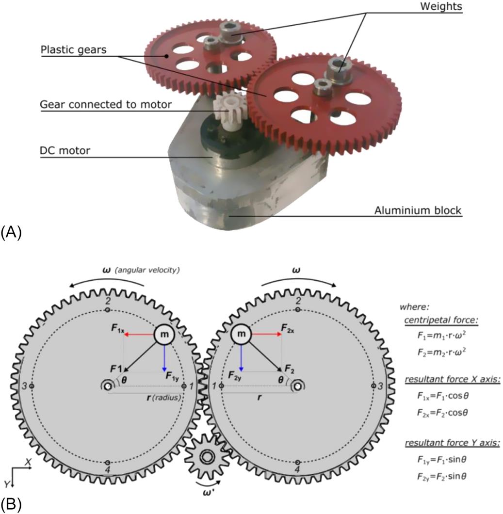
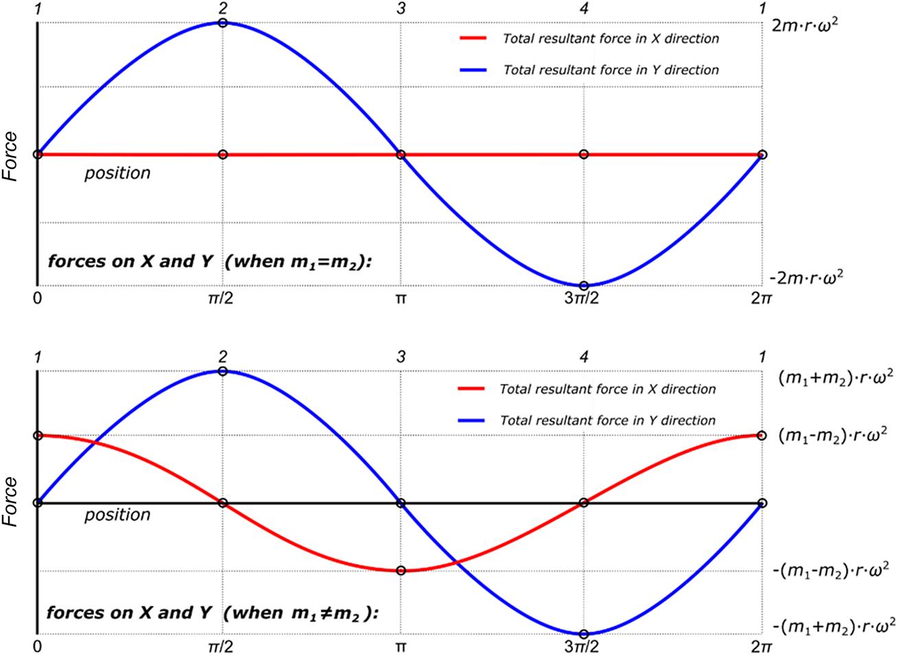
It may be noted that the excitation force produced by this device is dependent on three variables: mass of the weights attached to the gears (m), the radius of the gears (r), and the angular velocity of the gears (ω). The frequency (Hz) of the cyclic loading depends mainly on the angular velocity which can be easily controlled by the voltage (V) of the power supply. In order to control the force in Y axis, the appropriate masses should be attached to the rotating gears, considering the fact that the radius remains the same. Also it is possible to change the frequency and the amplitude by just replacing the type and the diameter of the gears. Once the amplitude and the frequency of the cyclic loads are defined, the device is mounted on the tower to simulate the desired overturning moment at the level of the foundation.
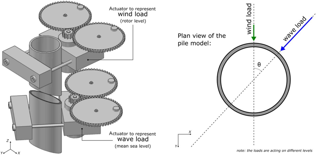
In a typical offshore project, the largest contribution toward the overturning moment is due to the wind and the wave loads having different magnitude of overturning moment, frequency, and also the number of cycles. A way to address this loading complexity in a scaled model tests is by attaching two of these eccentric mass actuators, one to represent each load (frequency and amplitude) and placing them at the correct height in order to produce the desired scaled bending moment at the base of the model. The result of such an arrangement would provide realistic results of the foundation’s long-term performance. Such a configuration is presented schematically in Fig. 17.8, where the wind and the wave are both acting along the same direction, i.e., collinear. There can be loading scenarios, when the wind and the wave may not be aligned and Fig. 17.9 shows a possible configuration that can be used for simulation.

Typical results presented by Lombardi et al. [8] highlighted that the long-term behavior of OWTs supported on monopiles is strongly affected by the level of strain generated in the soil adjacent the foundation (given in Eq. 17.3), whereby larger strains result in higher variation in foundation stiffness and natural frequency of the system. Evidently, the potential change in vibration characteristics has to be appropriately taken into account in design and prediction of the long-term performance of OWTs.
17.4 Scaling Laws for OWTs Supported on Multipod Foundations
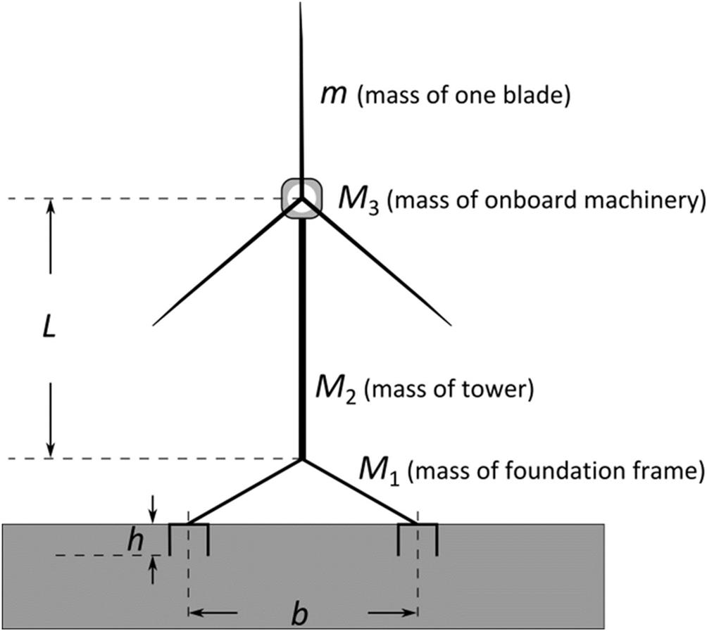
Offshore wind farm projects are increasingly turning to alternative foundations [13], which include jacket and multipod foundations. The scaling relations required to investigate such foundations need to take into account the geometric arrangement (i.e., characterizing the asymmetry). Thus, this section of the chapter incorporates the additional scaling laws required to study generic multipod foundations, such as the one depicted in Fig. 17.10.
The rules of similarity between the model and prototype that need to be maintained are as follows.
The dimensions of the small-scale model need to be chosen in such a way that similar modes of vibration will be excited in model and prototype. It is expected that rocking modes will govern the multipod (tripod or tetrapod suction piles or caissons) foundation and as a result relative spacing of individual pod foundations (b in Fig. 17.10) with respect to the tower height (L in Fig. 17.10) needs to be maintained (see Eq. (17.18)). This geometrical scaling is also necessary to determine the point of application of the resultant force on the model. The aspect ratio of the caisson (diameter-to-depth ratio) should also be maintained to ensure the pore water flow is reproduced. This leads to the similitude relationship given in Eq. (17.19).
(17.18)
where L is the length of the tower and b is the spacing of the caissons.
(17.19)
where D is the diameter of the caisson and h is the depth of the caisson.
To model the vibration of the tower, the mass distribution between the different components needs to be preserved. In other words, the ratios ![]() in Fig. 17.10 need to be maintained in model and prototype.
in Fig. 17.10 need to be maintained in model and prototype.
(17.20)
The relative stiffness between suction caisson and the surrounding soil: The stiffness of the caissons relative to the soil needs to be preserved in the model so that the caisson interacts similarly with the soil as in the prototype. Caisson flexibility affects both the dynamics and the soil–structure interaction and as a result this mechanism is of particular interest. Based on the work of Doherty et al. [14], the nondimensional flexibility of a suction caisson is given by:
(17.21)
where ![]() is the elastic modulus of caisson skirt (GPa);
is the elastic modulus of caisson skirt (GPa); ![]() is the thickness of caisson skirt (mm);
is the thickness of caisson skirt (mm); ![]() is the shear modulus of surrounding soil (GPa); and
is the shear modulus of surrounding soil (GPa); and ![]() is the diameter of the caisson (m).
is the diameter of the caisson (m).
The above group can be derived from the expression of hoop stress (![]() ) developed in a thin walled cylindrical pressure vessel given in Eq. (16.5).
) developed in a thin walled cylindrical pressure vessel given in Eq. (16.5).
(17.22)
noting that ![]() is the stress in the caisson which is proportional to the elastic modulus of caisson skirt (
is the stress in the caisson which is proportional to the elastic modulus of caisson skirt (![]() ) and
) and ![]() is the pressure applied by the soil, dependent on the shear modulus. Therefore the following relationship should be maintained:
is the pressure applied by the soil, dependent on the shear modulus. Therefore the following relationship should be maintained:
(17.23)
The loading encountered in a single caisson in a multipod foundation is a combination of vertical and horizontal load. For a combination of lateral and vertical load, a failure envelope given in Eq. (17.24) is often used in practice.
(17.24)
where ![]() is the bearing capacity in horizontal direction;
is the bearing capacity in horizontal direction; ![]() is the bearing capacity in vertical direction;
is the bearing capacity in vertical direction; ![]() is the vertical load on the individual caisson; and
is the vertical load on the individual caisson; and ![]() is the horizontal load on the caisson with
is the horizontal load on the caisson with ![]() =
=![]() =3 (see Ref. [7]).
=3 (see Ref. [7]).
The nondimensional group to preserve is ![]() which is proportional to
which is proportional to ![]() for sandy soil where
for sandy soil where ![]() is the buoyant soil unit weight (kN m−3) and D is the caisson diameter. The relationship for clay soil is given in Eq. (17.25c). Therefore the following relationship should hold:
is the buoyant soil unit weight (kN m−3) and D is the caisson diameter. The relationship for clay soil is given in Eq. (17.25c). Therefore the following relationship should hold:
(17.25a)
(17.25b)
(17.25c)
Details of the derivation are provided in Ref. [7]. The lateral load acting on the caisson can be derived from the CSR in the shear zone next to the footing which is quite similar to the case for pile as derived in earlier for the monopile due to the fact that caissons and monopiles will act as a rigid body. This leads us to a nondimensional group (Eq. (17.26)) that must be satisfied.
(17.26)
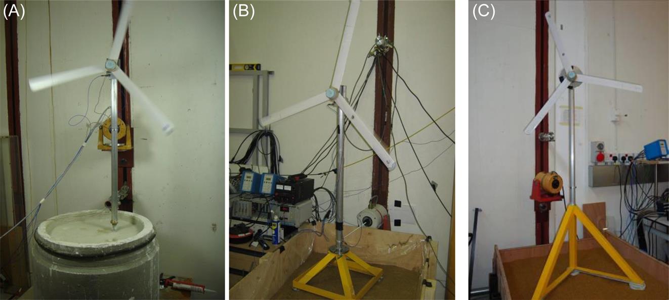
17.4.1 Typical Experimental Setups and Results
A series of tests were carried by Bhattacharya et al. [13] to investigate the dynamics and long-term performance of small-scale OWTs models supported on multipod foundations (Fig. 17.11). Fig. 17.12 shows the asymmetric model arrangement in a typical setup. The results showed that the multipod foundations (symmetric or asymmetric) exhibit two closely spaced natural frequencies corresponding to the rocking modes of vibration in two principle axes. Furthermore, the corresponding two spectral peaks change with repeated cycles of loading and they converge for symmetric tetrapods but not for asymmetric tripods. From the fatigue design point of view, the two spectral peaks for multipod foundations broaden the range of frequencies that can be excited by the broadband nature of the environmental loading (wind and wave) thereby impacting the extent of motions. Thus the system life span (number of cycles to failure) may effectively increase for symmetric foundations as the two peaks will tend to converge. However, for asymmetric foundations, the system life may continue to be affected adversely as the two peaks will not converge. In this sense, designers should prefer symmetric foundations to asymmetric foundations.

17.5 Conclusions
This chapter shows that small-scale experimental studies can be carried out to study complex dynamic soil–structure interaction problems where there is no prior information. The long-term performance of OWTs has been studied because there is a real concern regarding the effect on performance of changes in the foundation stiffness.
Mechanics-based nondimensional groups have been derived in order to study the various aspects of this problem and their validity has been verified using physical modeling.