Chapter 4. Radio Communication Basics

In this chapter on radio communication basics, we first will take a look at the phenomena that lets us transfer information from one point to another without any physical medium—the propagation of radio waves. If you want to design an efficient radio communication system, even for operation over relatively short distances, you should understand the behavior of the wireless channel in the various surroundings where this communication is to take place. While the use of “brute force”—increasing transmission power—could overcome inordinate path losses, limitations imposed on design by required battery life, or by regulatory authorities, make it imperative to develop and deploy short-range radio systems using solutions that a knowledge of radio propagation can give.

The overall behavior of radio waves is described by Maxwell's equations. In 1873, the British physicist James Clerk Maxwell published his Treatise on Electricity and Magnetism in which he presented a set of equations that describe the nature of electromagnetic fields in terms of space and time. Heinrich Rudolph Hertz performed experiments to confirm Maxwell's theory, which led to the development of wireless telegraph and radio. Maxwell's equations form the basis for describing the propagation of radio waves in space, as well as the nature of varying electric and magnetic fields in conducting and insulating materials, and the flow of waves in waveguides. From them, you can derive the skin effect equation and the electric and magnetic field relationships very close to antennas of all kinds. A number of computer programs on the market, based on the solution of Maxwell's equations, help in the design of antennas, anticipate electromagnetic radiation problems from circuit board layouts, calculate the effectiveness of shielding, and perform accurate simulation of ultra-high-frequency and microwave circuits. While you don't have to be an expert in Maxwell's equations to use these programs (you do in order to write them!), having some familiarity with the equations may take the mystery out of the operation of the software and give an appreciation for its range of application and limitations.

4.1. Mechanisms of Radio Wave Propagation

Radio waves can propagate from transmitter to receiver in four ways: through ground waves, sky waves, free space waves, and open field waves.

Ground waves exist only for vertical polarization, produced by vertical antennas, when the transmitting and receiving antennas are close to the surface of the earth. The transmitted radiation induces currents in the earth, and the waves travel over the earth's surface, being attenuated according to the energy absorbed by the conducting earth. The reason that horizontal antennas are not effective for ground wave propagation is that the horizontal electric field that they create is short circuited by the earth. Ground wave propagation is dominant only at relatively low frequencies, up to a few megahertz, so it needn't concern us here.

Sky wave propagation is dependent on reflection from the ionosphere, a region of rarified air high above the earth's surface that is ionized by sunlight (primarily ultraviolet radiation). The ionosphere is responsible for long-distance communication in the high-frequency bands between 3 and 30 MHz. It is very dependent on time of day, season, longitude on the earth, and the multi-year cyclic production of sunspots on the sun. It makes possible long-range communication using very low-power transmitters. Most short-range communication applications use VHF, UHF, and microwave bands, generally above 40 MHz. There are times when ionospheric reflection occurs at the low end of this range, and then sky wave propagation can be responsible for interference from signals originating hundreds of kilometers away. However, in general, sky wave propagation does not affect the short-range wireless applications that we are interested in.

The most important propagation mechanism for short-range communication on the VHF and UHF bands is that which occurs in an open field, where the received signal is a vector sum of a direct line-of-sight signal and a signal from the same source that is reflected off the earth. We discuss below the relationship between signal strength and range in line-of-sight and open-field topographies.

The range of line-of-sight signals, when there are no reflections from the earth or ionosphere, is a function of the dispersion of the waves from the transmitter antenna. In this free-space case the signal strength decreases in inverse proportion to the distance away from the transmitter antenna. When the radiated power is known, the field strength is given by equation (4-1):(4-1)

where P^t is the transmitted power, G^t is the antenna gain, and d is the distance. When P^t is in watts and d is in meters, E is volts/meter.

To find the power at the receiver (P^r ) when the power into the transmitter antenna is known, use (4-2):(4-2)

G^t and G^r are the transmitter and receiver antenna gains, and λ is the wavelength.

Range can be calculated on this basis at high UHF and microwave frequencies when high-gain antennas are used, located many wavelengths above the ground. Signal strength between the earth and a satellite, and between satellites, also follows the inverse distance law, but this case isn't in the category of short-range communication! At microwave frequencies, signal strength is also reduced by atmospheric absorption caused by water vapor and other gases that constitute the air.

4.2. Open Field Propagation

Although the formulas in the previous section are useful in some circumstances, the actual range of a VHF or UHF signal is affected by reflections from the ground and surrounding objects. The path lengths of the reflected signals differ from that of the line-of-sight signal, so the receiver sees a combined signal with components having different amplitudes and phases. The reflection causes a phase reversal. A reflected signal having a path length exceeding the line-of-sight distance by exactly the signal wavelength or a multiple of it will almost cancel completely the desired signal (“almost” because its amplitude will be slightly less than the direct signal amplitude). On the other hand, if the path length of the reflected signal differs exactly by an odd multiple of half the wavelength, the total signal will be strengthened by “almost” two times the free space direct signal.

In an open field with flat terrain there will be no reflections except the unavoidable one from the ground. It is instructive and useful to examine in depth the field strength versus distance in this case.”

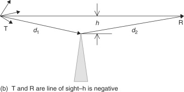
In Figure 4.1 we see transmitter and receiver antennas separated by distance d and situated at heights h¹ and h². Using trigonometry, we can find the line of sight and reflected signal path lengths d¹ and d². Just as in optics, the angle of incidence equals the angle of reflection θ. We get the relative strength of the direct signal and reflected signal using the inverse path length relationship. If the ground were a perfect mirror, the relative reflected signal strength would exactly equal the inverse of d². In this case, the reflected signal phase would shift 180 degrees at the point of reflection. However, the ground is not a perfect reflector. Its characteristics as a reflector depend on its conductivity, permittivity, the polarization of the signal and its angle of incidence. Accounting for polarization, angle of incidence, and permittivity, we can find the reflection coefficient, which approaches −1 as the distance from the transmitter increases. The signals reaching the receiver are represented as complex numbers since they have both phase and amplitude. The phase is found by subtracting the largest interval of whole wavelength multiples from the total path length and multiplying the remaining fraction of a wavelength by 2π radians, or 360 degrees.

Figure 4.1. Open field signal paths

Figure 4.2 gives a plot of relative open field signal strength versus distance using the following parameters:

Figure 4.2. Field strength vs. range at 300 MHz

Polarity—horizontal

Frequency—300 MHz

Antenna heights—both 3 meters

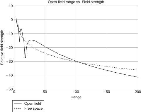
Relative ground permittivity—15

Also shown is a plot of free space field strength versus distance (dotted line). In both plots, signal strength is referenced to the free space field strength at a range of 3 meters.

Notice in Figure 4.2 that, up to a range of around 50 meters, there are several sharp depressions of field strength, but the signal strength is mostly higher than it would be in free space. Beyond 100 meters, signal strength decreases more rapidly than for the free space model. Whereas there is an inverse distance law for free space, in the open field beyond 100 meters (for these parameters) the signal strength follows an inverse square law. Increasing the antenna heights extends the distance at which the inverse square law starts to take effect. This distance, d^m, can be approximated by(4-3)

where h¹ and h² are the transmitting and receiving antenna heights above ground and λ is the wavelength, all in the same units as the distance d^m.

In plotting Figure 4.2, we assumed horizontal polarization. Both antenna heights, h¹ and h², are 3 meters. When vertical polarization is used, the extreme local variations of signal strengths up to around 50 meters are reduced, because the ground reflection coefficient is less at larger reflection angles. However, for both polarizations, the inverse square law comes into effect at approximately the same distance. This distance in Figure 4.2 where λ is 1 meter is, from Eq. (4-3): d^m=(12×3×3)/λ=108 meters. In Figure 4.2 we see that this is approximately the distance where the open-field field strength falls below the free-space field strength.

4.3. Diffraction

Diffraction is a propagation mechanism that permits wireless communication between points where there is no line-of-sight path due to obstacles that are opaque to radio waves. For example, diffraction makes it possible to communicate around the earth's curvature, as well as beyond hills and obstructions. It also fills in the spaces around obstacles when short-range radio is used inside buildings. Figure 4.3 is an illustration of diffraction geometries, showing an obstacle whose extremity has the shape of a knife edge. The obstacle should be seen as a half plane whose dimension is infinite into and out of the paper. The field strength at a receiving point relative to the free-space field strength without the obstacle is the diffraction gain. The phenomenon of diffraction is due to the fact that each point on the wave front emanating from the transmitter is a source of a secondary wave emission. Thus, at the knife edge of the obstacle, as shown in Figure 4.3a, there is radiation in all directions, including into the shadow.

Figure 4.3. Knife-edge diffraction geometry

The diffraction gain depends in a rather complicated way on a parameter that is a function of transmitter and receiver distances from the obstacle, d¹ and d², the obstacle dimension h, and the wavelength. Think of the effect of diffraction in an open space in a building where a wide metal barrier extending from floor to ceiling exists between the transmitter and the receiver. In our example, the space is 12 meters wide and the barrier is 6 meters wide, extending to the right side. When the transmitter and receiver locations are fixed on a line at a right angle to the barrier, the field strength at the receiver depends on the perpendicular distance from the line-of-sight path to the barrier's edge. Figure 4.4 is a plot of diffraction gain when transmitter and receiver are each 10 meters from the edge of the obstruction and on either side of it. The dimension “h” varies between −6 meters and 6 meters—that is, from the left side of the space where the dimension “h” is considered negative, to the right side where “h” is positive and fully in the shadow of the barrier. Transmission frequency for the plot is 300 MHz. Note that the barrier affects the received signal strength even when there is a clear line of sight between the transmitter and receiver (“h” is negative as shown in Figure 4.3b). When the barrier edge is on the line of sight, diffraction gain is approximately −6 dB, and as the line-of-sight path gets farther from the barrier (to the left in this example), the signal strength varies in a cyclic manner around 0 dB gain. As the path from transmitter to receiver gets farther from the barrier edge into the shadow, the signal attenuation increases progressively.

Figure 4.4. Example plot of diffraction gain vs. “h”

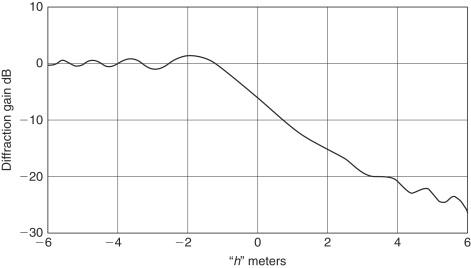
Admittedly, the situation depicted in Figure 4.4 is idealistic, since it deals with only one barrier of very large extent. Normally there are several partitions and other obstacles near or between the line of sight path and a calculation of the diffraction gain would be very complicated, if not impossible. However, a knowledge of the idealistic behavior of the defraction gain and its dependence on distance and frequency can give qualitative insight.

4.4. Scattering

A third mechanism affecting path loss, after reflection and diffraction, is scattering. Rough surfaces in the vicinity of the transmitter do not reflect the signal cleanly in the direction determined by the incident angle, but diffuse it, or scatter it in all directions. As a result, the receiver has access to additional radiation and path loss may be less than it would be from considering reflection and diffraction alone.

The degree of roughness of a surface and the amount of scattering it produces depends on the height of the protuberances on the surface compared to a function of the wavelength and the angle of incidence. The critical surface height h^c is given by [Gibson, p. 360](4-4)

where λ is the wavelength and θⁱ is the angle of incidence. It is the dividing line between smooth and rough surfaces when applied to the difference between the maximum and the minimum protuberances.

4.5. Path Loss

The numerical path loss is the ratio of the total radiated power from a transmitter antenna times the numerical gain of the antenna in the direction of the receiver to the power available at the receiver antenna. This is the ratio of the transmitter power delivered to a lossless antenna with numerical gain of 1 (0 dB) to that at the output of a 0 dB gain receiver antenna. Sometimes, for clarity, the ratio is called the isotropic path loss. An isotropic radiator is an ideal antenna that radiates equally in all directions and therefore has a gain of 0 dB. The inverse path loss ratio is sometimes more convenient to use. It is called the path gain and when expressed in decibels is a negative quantity. In free space, the isotropic path gain PG is derived from (4-2), resulting in(4-5)

We have just examined several factors that affect the path loss of VHF-UHF signals—ground reflection, diffraction, and scattering. For a given site, it would be very difficult to calculate the path loss between transmitters and receivers, but empirical observations have allowed some general conclusions to be drawn for different physical environments. These conclusions involve determining the exponent, or range of exponents, for the distance d related to a short reference distance d⁰. We then can write the path gain as dependent on the exponent n:(4-6)

where k is equal to the path gain when d=d⁰. Table 4.1 shows path loss for different environments.

Table 4.1. Path loss exponents for different environments [Gibson, p. 362]

Environment	Path gain exponent
Free space	2
Open field (long distance)	4
Cellular radio — urban area	2.7–4
Shadowed urban cellular radio	5–6
In building line of sight	1.6–1.8
In building — obstructed	4–6

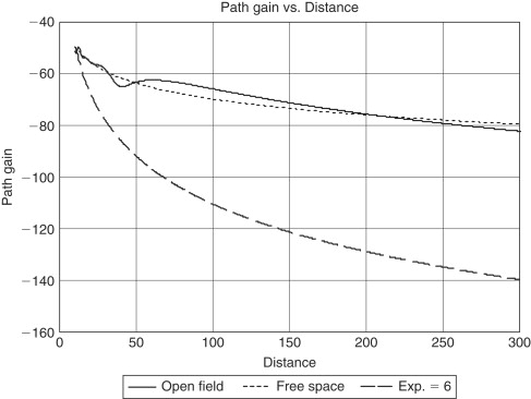
As an example of the use of the path gain exponent, let's assume the open field range of a security system transmitter and receiver is 300 meters. What range can we expect for their installation in a building?

Figure 4.5 shows curves of path gain versus distance for free-space propagation, open field propagation, and path gain with exponent 6, a worst case taken from Table 4.1 for “In building, obstructed.” Transmitter and receiver heights are 2.5 meters, polarization is vertical, and the frequency is 915 MHz. The reference distance is 10 meters, and for all three curves the path gain at 10 meters is taken to be that of free space. For an open field distance of 300 meters, the path gain is −83 dB. The distance on the curve with exponent n=6 that gives the same path gain is 34 meters. Thus, a wireless system that has an outdoor range of 300 meters may be effective only over a range of 34 meters, on the average, in an indoor installation.

Figure 4.5. Path gain

The use of an empirically derived relative path loss exponent gives an estimate for average range, but fluctuations around this value should be expected. The next section shows the spread of values around the mean that occurs because of multipath radiation.

4.6. Multipath Phenomena

We have seen that reflection of a signal from the ground has a significant effect on the strength of the received signal. The nature of short-range radio links, which are very often installed indoors and use omnidirectional antennas, makes them accessible to a multitude of reflected rays, from floors, ceilings, walls, and the various furnishings and people that are invariably present near the transmitter and receiver. Thus, the total signal strength at the receiver is the vector sum of not just two signals, as we studied in Section 4.2, but of many signals traveling over multiple paths. In most cases indoors, there is no direct line-of-sight path, and all signals are the result of reflection, diffraction and scattering.

From the point of view of the receiver, there are several consequences of the multipath phenomena.

• Variation of signal strength. Phase cancellation and strengthening of the resultant received signal causes an uncertainty in signal strength as the range changes, and even at a fixed range when there are changes in furnishings or movement of people. The receiver must be able to handle the considerable variations in signal strength.
• Frequency distortion. If the bandwidth of the signal is wide enough so that its various frequency components have different phase shifts on the various signal paths, then the resultant signal amplitude and phase will be a function of sideband frequencies. This is called frequency selective fading.
• Time delay spread. The differences in the path lengths of the various reflected signals causes a time delay spread between the shortest path and the longest path. The resulting distortion can be significant if the delay spread time is of the order of magnitude of the minimum pulse width contained in the transmitted digital signal. There is a close connection between frequency selective fading and time-delay distortion, since the shorter the pulses, the wider the signal bandwidth. Measurements in factories and other buildings have shown multipath delays ranging from 40 to 800 ns (Gibson, p. 366).
• Fading. When the transmitter or receiver is in motion, or when the physical environment is changing (tree leaves fluttering in the wind, people moving around), there will be slow or rapid fading, which can contain amplitude and frequency distortion, and time delay fluctuations. The receiver AGC and demodulation circuits must deal properly with these effects.

4.7. Flat Fading

In many of the short-range radio applications covered in this book, the signal bandwidth is narrow and frequency distortion is negligible. The multipath effect in this case is classified as flat fading. In describing the variation of the resultant signal amplitude in a multipath environment, we distinguish two cases: (1) there is no line-of-sight path and the signal is the resultant of a large number of randomly distributed reflections; (2) the random reflections are superimposed on a signal over a dominant constant path, usually the line of sight.

Short-range radio systems that are installed indoors or outdoors in built-up areas are subject to multipath fading essentially of the first case. Our aim in this section is to determine the signal strength margin that is needed to ensure that reliable communication can take place at a given probability. While in many situations there will be a dominant signal path in addition to the multipath fading, restricting ourselves to an analysis of the case where all paths are the result of random reflections gives us an upper bound on the required margin.

4.7.1. Rayleigh Fading

The first case can be described by a received signal R(t), expressed as(4-7)

where r and θ are random variables for the peak signal, or envelope, and phase. Their values may vary with time, when various reflecting objects are moving (people in a room, for example), or with changes in position of the transmitter or receiver which are small in respect to the distance between them. We are not dealing here with the large-scale path gain that is expressed in Eq. (4-5) and (4-6). For simplicity, Eq. (4-7) shows a CW (continuous wave) signal as the modulation terms are not needed to describe the fading statistics.

The envelope of the received signal, r, can be statistically described by the Rayleigh distribution whose probability density function is(4-8)

where σ² represents the variance of R(t) in Eq. (4-7), which is the average received signal power. This function is plotted in Figure 4.6. We normalized the curve with σ equal to 1.In this plot, the average value of the signal envelope, shown by a dotted vertical line, is 1.253. Note that it is not the most probable value, which is 1 (σ). The area of the curve between any two values of signal strength r represents the probability that the signal strength will be in that range. The average for the Rayleigh distribution, which is not symmetric, does not divide the curve area in half. The parameter that does this is the median, which in this case equals 1.1774. There is a 50% probability that a signal will be below the median and 50% that it will be above.

Figure 4.6. Rayleigh probability density function

As stated above, the Rayleigh distribution is used to determine the signal margin required to give a desired communication reliability over a fading channel with no line of sight. The curve labeled “1 Channel” in Figure 4.7 is a cumulative distribution function with logarithmic axes. For any point on the curve, the probability of fading below the margin indicated on the abscissa is given as the ordinate. The curve is scaled such that “0 dB” signal margin represents the point where the received signal equals the mean power of the fading signal, σ², making the assumption that the received signal power with no fading equals the average power with fading. Some similar curves in the literature use the median power, or the power corresponding to the average envelope signal level, r^a, as the reference, “0 dB” value.

Figure 4.7. Fading margins

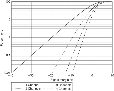
An example of using the curve is as follows. Say you require a communication reliability of 99%. Then the minimum usable signal level is that for which there is a 1% probability of fading below that level. On the curve, the margin corresponding to 1% is 20 dB.Thus, you need a signal strength 20 dB larger than the required signal if there was no fading. Assume you calculated path loss and found that you need to transmit 4 mW to allow reception at the receiver's sensitivity level. Then, to ensure that the signal will be received 99% of the time during fading, you'll need 20 dB more power or 6 dBm (4 mW) plus 20 dB equals 26 dBm or 400 mW. If you don't increase the power, you can expect loss of communication 63% of the time, corresponding to the “0 dB” margin point on the “Channel 1” curve of Figure 4.7.

Table 4.2 shows signal margins for different reliabilities.

Table 4.2. Signal margins for different reliabilities

Reliability, Percent	Fading Margin, dB
90	10
99	20
99.9	30
99.99	40

4.8. Diversity Techniques

Communication reliability for a given signal power can be increased substantially in a multipath environment through diversity reception. If signals are received over multiple, independent channels, the largest signal can be selected for subsequent processing and use. The key to this solution is the independence of the channels. The multipath effect of nulling and of strengthening a signal is dependent on transmitter and receiver spatial positions, on wavelength (or frequency) and on polarity. Let's see how we can use these parameters to create independent diverse channels.

4.8.1. Space Diversity

A signal that is transmitted over slightly different distances to a receiver may be received at very different signal strengths. For example, in Figure 4.2 the signal at 17 meters is at a null and at 11 meters at a peak. If we had two receivers, each located at one of those distances, we could choose the strongest signal and use it. In a true multipath environment, the source, receiver, or the reflectors may be constantly in motion, so the nulls and the peaks would occur at different times on each channel. Sometimes Receiver 1 has the strongest signal, at other times Receiver 2. Figure 4.8 illustrates the paths to two receivers from several reflectors. Although there may be circumstances where the signals at both receiver locations are at around the same level, when it doesn't matter which receiver output is chosen, most of the time one signal will be stronger than the other. By selecting the strongest output, the average output after selection will be greater than the average output of one channel alone. To increase even more the probability of getting a higher average output, we could use three or more receivers. From Figure 4.7 you can find the required fading margin using diversity reception having 2, 3, or 4 channels. Note that the plots in Figure 4.7 are based on completely independent channels. When the channels are not completely independent, the results will not be as good as indicated by the plots.

Figure 4.8. Space diversity

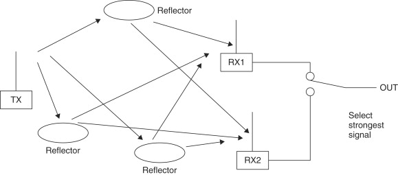
It isn't necessary to use complete receivers at each location, but separate antennas and front ends must be used, at least up to the point where the signal level can be discerned and used to decide on the switch position.

4.8.2. Frequency Diversity

You can get a similar differential in signal strength over two or more signal channels by transmitting on separate frequencies. For the same location of transmitting and receiving antennas, the occurrences of peaks and nulls will differ on the different frequency channels. As in the case of space diversity, choosing the strongest channel will give a higher average signal-to-noise ratio than on either one of the channels. The required frequency difference to get near independent fading on the different channels depends on the diversity of path lengths or signal delays. The larger the difference in path lengths, the smaller the required frequency difference of the channels.

4.8.3. Polarization Diversity

Fading characteristics are dependent on polarization. A signal can be transmitted and received separately on horizontal and vertical antennas to create two diversity channels. Reflections can cause changes in the direction of polarization of a radio wave, so this characteristic of a signal can be used to create two separate signal channels. Thus, cross-polarized antennas can be used at the receiver only. Polarization diversity can be particularly advantageous in a portable handheld transmitter, since the orientation of its antenna will not be rigidly defined.

Polarization diversity doesn't allow the use of more than two channels, and the degree of independence of each channel will usually be less than in the two other cases. However, it may be simpler and less expensive to implement and may give enough improvement to justify its use, although performance will be less than can be achieved with space or frequency diversity.

4.8.4. Diversity Implementation

In the descriptions above, we talked about selecting or switching to the channel having the highest signal level. A more effective method of using diversity is called “maximum ratio combining.” In this technique, the outputs of each independent channel are added together after the channel phases are made equal and channel gains are adjusted for equal signal levels. Maximum ratio combining is known to be optimum as it gives the best statistical reduction of fading of any linear diversity combiner. In applications where accurate amplitude estimation is difficult, the channel phases only may be equalized and the outputs added without weighting the gains. Performance in this case is almost as good as in maximum ratio combining. [Gibson, p. 170, 171]

Space diversity has the disadvantage of requiring significant antenna separation, at least in the VHF and lower UHF bands. In the case where multipath signals arrive from all directions, antenna spacing on the order of .5λ to .8λ is adequate in order to have reasonably independent, or decorrelated, channels. This is at least one-half meter at 300 MHz. When the multipath angle spread is small—for example, when directional antennas are used—much larger separations are required.

Frequency diversity eliminates the need for separate antennas, but the simultaneous use of multiple frequency channels entails increased total power and spectrum utilization. Sometimes data are repeated on different frequencies so that simultaneous transmission doesn't have to be used. Frequency separation must be adequate to create decorrelated channels. The bandwidths allocated for unlicensed short-range use are rarely adequate, particularly in the VHF and UHF ranges (transmitting simultaneously on two separate bands can and has been done). Frequency diversity to reduce the effects of time delay spread is achieved with frequency hopping or direct sequence spread spectrum modulation, but for the spreads encountered in indoor applications, the pulse rate must be relatively high—of the order of several megabits per second—in order to be effective. For long pulse widths, the delay spread will not be a problem anyway, but multipath fading will still occur and the amount of frequency spread normally used in these cases is not likely to solve it.

When polarity diversity is used, the orthogonally oriented antennas can be close together, giving an advantage over space diversity when housing dimensions relative to wavelength are small. Performance may not be quite as good, but may very well be adequate, particularly when used in a system having portable hand-held transmitters, which have essentially random polarization.

Although we have stressed that at least two independent (decorrelated) channels are needed for diversity reception, sometimes shortcuts are taken. In some low-cost security systems, for example, two receiver antennas—space diverse or polarization diverse—are commutated directly, usually by diode switches, before the front end or mixer circuits. Thus, a minimum of circuit duplication is required. In such applications the message frame is repeated many times, so if there happens to be a multipath null when the front end is switched to one antenna and the message frames are lost, at least one or more complete frames will be correctly received when the switch is on the other antenna, which is less affected by the null. This technique works for slow fading, where the fade doesn't change much over the duration of a transmission of message frames. It doesn't appear to give any advantage during fast fading, when used with moving hand-held transmitters, for example. In that case, a receiver with one antenna will have a better chance of decoding at least one of many frames than when switched antennas are used and only half the total number of frame repetitions are available for each. In a worst-case situation with fast fading, each antenna in turn could experience a signal null.

4.8.5. Statistical Performance Measure

We can estimate the performance advantage due to diversity reception with the help of Figure 4.7. Curves labeled “2 Channels” through “4 Channels” are based on the selection combining technique.

Let's assume, as before, that we require communication reliability of 99 percent, or an error rate of 1 percent. From probability theory the probability that two independent channels would both have communication errors is the product of the error probabilities of each channel. Thus, if each of two channels has an error probability of 10 percent, the probability that both channels will have signals below the sensitivity threshold level when selection is made is .1 times .1, which equals .01, or 1 percent. This result is reflected in the curve “2 Channels”. We see that the signal margin needed for 99 percent reliability (1 percent error) is 10 dB. Using diversity reception with selection from two channels allows a reliability margin of only 10 dB instead of 20 dB, which is required if there is no diversity. Continuing the previous example, we need to transmit only 40 mW for 99 percent reliability instead of 400 mW. Required margins by selection among three channels and four channels is even less—6 dB and 4 dB, respectively.

Remember that the reliability margins using selection combining diversity as shown in Figure 4.7 are ideal cases, based on the Rayleigh fading probability distribution and independently fading channels. However, even if these premises are not realized in practice, the curves still give us approximations of the improvement that diversity reception can bring.

4.9. Noise

The ultimate limitation in radio communication is not the path loss or the fading. Weak signals can be amplified to practically any extent, but it is the noise that bounds the range we can get or the communication reliability that we can expect from our radio system. There are two sources of receiver noise—interfering radiation that the antenna captures along with the desired signal, and the electrical noise that originates in the receiver circuits. In either case, the best signal-to-noise ratio will be obtained by limiting the bandwidth to what is necessary to pass the information contained in the signal. A further improvement can be had by reducing the receiver noise figure, which decreases the internal receiver noise, but this measure is effective only as far as the noise received through the antenna is no more than about the same level as the receiver noise. Finally, if the noise can be reduced no further, performance of digital receivers can be improved by using error correction coding up to a point, which is designated as channel capacity. The capacity is the maximum information rate that the specific channel can support, and above this rate communication is impossible. The channel capacity is limited by the noise density (noise power per hertz) and the bandwidth.

Figure 4.9 shows various sources of noise over a frequency range of 20 kHz up to 10 GHz. The strength of the noise is shown in microvolts/meter for a bandwidth of 10 kHz, as received by a half-wave dipole antenna at each frequency. The curve labeled “equivalent receiver noise” translates the noise generated in the receiver circuits into an equivalent field strength so that it can be compared to the external noise sources. Receiver noise figures on which the curve is based vary in a log-linear manner with 2 dB at 50 MHz and 9 dB at 1 GHz. The data in Figure 4.9 are only a representative example of radiation and receiver noise, taken at a particular time and place.

Figure 4.9. External noise sources

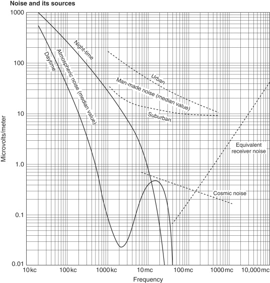
(Reference Data for Radio Engineers, Fourth Edition)

Note that all of the noise sources shown in Figure 4.9 are dependent on frequency. The relative importance of the various noise sources to receiver sensitivity depends on their strength relative to the receiver noise. Atmospheric noise is dominant on the low radio frequencies but is not significant on the bands used for short-range communication—above around 40 MHz. Cosmic noise comes principally from the sun and from the center of our galaxy. In the figure, it is masked out by man-made noise, but in locations where man-made noise is a less significant factor, cosmic noise affects sensitivity up to 1 GHz.

Man-made noise is dominant in the range of frequencies widely used for short-range radio systems—VHF and low to middle UHF bands. It is caused by a wide range of ubiquitous electrical and electronic equipment, including automobile ignition systems, electrical machinery, computing devices and monitors. While we tend to place much importance on the receiver sensitivity data presented in equipment specifications, high ambient noise levels can make the sensitivity irrelevant in comparing different devices. For example, a receiver may have a laboratory measured sensitivity of −105 dBm for a signal-to-noise ratio of 10 dB. However, when measured with its antenna in a known electric field and accounting for the antenna gain, −95 dBm may be required to give the same signal-to-noise ratio.

From around 800 MHz and above, receiver sensitivity is essentially determined by the noise figure. Improved low-noise amplifier discrete components and integrated circuit blocks produce much better noise figures than those shown in Figure 4.9 for high UHF and microwave frequencies. Improving the noise figure must not be at the expense of other characteristics—intermodulation distortion, for example, which can be degraded by using a very high-gain amplifier in front of a mixer to improve the noise figure. Intermodulation distortion causes the production of inband interfering signals from strong signals on frequencies outside of the receiving bandwidth.

External noise will be reduced when a directional antenna is used. Regulations on unlicensed transmitters limit the peak radiated power. When possible, it is better to use a high-gain antenna and lower transmitter power to achieve the same peak radiated power as with a lower gain antenna. The result is higher sensitivity through reduction of external noise. Manmade noise is usually less with a horizontal antenna than with a vertical antenna.

4.10. Communication Protocols and Modulation

A simple block diagram of a digital wireless link is shown in Figure 4.10. The link transfers information originating at one location, referred to as source data, to another location where it is referred to as reconstructed data. A more concrete implementation of a wireless system, a security system, is shown in Figure 4.11.

Figure 4.10. Radio communication link diagram

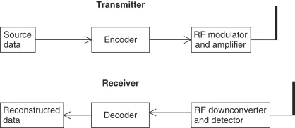
Figure 4.11. Security system

4.10.1. Baseband Data Format and Protocol

Let's first take a look at what information we may want to transfer to the other side. This is important in determining what bandwidth the system needs.

4.10.1.1. Change-of-State Source Data

Many short-range systems only have to relay information about the state of a contact. This is true of the security system of Figure 4.11 where an infrared motion detector notifies the control panel when motion is detected. Another example is the push-button transmitter, which may be used as a panic button or as a way to activate and deactivate the control system, or a wireless smoke detector, which gives advance warning of an impending fire. There are also what are often referred to as “technical” alarms—gas detectors, water level detectors, and low and high temperature detectors—whose function is to give notice of an abnormal situation.

All these examples are characterized as very low-bandwidth information sources. Change of state occurs relatively rarely, and when it does, we usually don't care if knowledge of the event is signaled tens or even hundreds of milliseconds after it occurs. Thus, required information bandwidth is very low—several hertz.

It would be possible to maintain this very low bandwidth by using the source data to turn on and off the transmitter at the same rate the information occurs, making a very simple communication link. This is not a practical approach, however, since the receiver could easily mistake random noise on the radio channel for a legitimate signal and thereby announce an intrusion, or a fire, when none occurred. Such false alarms are highly undesirable, so the simple on/off information of the transmitter must be coded to be sure it can't be misinterpreted at the receiver.

This is the purpose of the encoder shown in Figure 4.10. This block creates a group of bits, assembled into a frame, to make sure the receiver will not mistake a false occurrence for a real one. Figure 4.12 is an example of a message frame. The example has four fields. The first field is a preamble with start bit, which conditions the receiver for the transfer of information and tells it when the message begins. The next field is an identifying address. This address is unique to the transmitter and its purpose is to notify the receiver from where, or from what unit, the message is coming. The data field follows, which may indicate what type of event is being signaled, followed, in some protocols, by a parity bit or bits to allow the receiver to determine whether the message was received correctly.

Figure 4.12. Message frame

Address Field

The number of bits in the address field depends on the number of different transmitters there may be in the system. Often the number of possibilities is far greater than this, to prevent confusion with neighboring, independent systems and to prevent the statistically possible chance that random noise will duplicate the address. The number of possible addresses in the code is 2^L1, where L1 is the length of the message field. In many simple security systems the address field is determined by dip switches set by the user. Commonly, eight to ten dip switch positions are available, giving 256 to 1024 address possibilities. In other systems, the address field, or device identity number, is a code number set in the unit micro-controller during manufacture. This code number is longer than that produced by dip switches, and may be 16 to 24 bits long, having 65,536 to 16,777,216 different codes. The longer codes greatly reduce the chances that a neighboring system or random event will cause a false alarm. On the other hand, the probability of detection is lower with the longer code because of the higher probability of error. This means that a larger signal-to-noise ratio is required for a given probability of detection.

In all cases, the receiver must be set up to recognize transmitters in its own system. In the case of dip-switch addressing, a dip switch in the receiver is set to the same address as in the transmitter. When several transmitters are used with the same receiver, all transmitters must have the same identification address as that set in the receiver. In order for each individual transmitter to be recognized, a subfield of two to four extra dip switch positions can be used for this differentiation. When a built-in individual fixed identity is used instead of dip switches, the receiver must be taught to recognize the identification numbers of all the transmitters used in the system; this is done at the time of installation. Several common ways of accomplishing this are:

• Wireless “learn” mode. During a special installation procedure, the receiver stores the addresses of each of the transmitters which are caused to transmit during this mode;
• Infrared transmission. Infrared emitters and detectors on the transmitter and receiver, respectively, transfer the address information;
• Direct key-in. Each transmitter is labeled with its individual address, which is then keyed into the receiver or control panel by the system installer;
• Wired learn mode. A short cable temporarily connected between the receiver and transmitter is used when performing the initial address recognition procedure during installation.

Advantages and Disadvantages of the Two Addressing Systems

Some advantages and disadvantages of the two types of addressing system are shown in Tables 4.3 and 4.4. Table 4.3 shows dip switch addressing and Table 4.4 shows internal fixed code identity addressing.

Table 4.3. Dip switch

Advantages	Disadvantages
Unlimited number of transmitters can be used with a receiver.	Limited number of bits increases false alarms and interference from adjacent systems.
Can be used with commercially available data encoders and decoders.	Device must be opened for coding during installation.
Transmitter or receiver can be easily replaced without recoding the opposite terminal.	Multiple devices in a system are not distinguishable in most simple systems.
	Control systems are vulnerable to unauthorized operation since the address code can be duplicated by trial and error.

Table 4.4. Internal fixed code identity

Advantages	Disadvantages
Large number of code bits reduces possibility of false alarms.	Longer code reduces probability of detection.
System can be set up without opening transmitter.	Replacing transmitter or receiver involves redoing the code learning procedure.
Each transmitter is individually recognized by receiver.	Limited number of transmitters can be used with each receiver.
	Must be used with a dedicated microcontroller. Cannot be used with standard encoders and decoders.

Code-hopping Addressing

While using a large number of bits in the address field reduces the possibility of false identification of a signal, there is still a chance of purposeful duplication of a transmitter code to gain access to a controlled entry. Wireless push buttons are used widely for access control to vehicles and buildings. Radio receivers exist, popularly called “code grabbers,” which receive the transmitted entry signals and allow retransmitting them for fraudulent access to a protected vehicle or other site. To counter this possibility, addressing techniques were developed that cause the code to change every time the push button is pressed, so that even if the transmission is intercepted and recorded, its repetition by a would-be intruder will not activate the receiver, which is now expecting a different code. This method is variously called code rotation, code hopping, or rolling code addressing. In order to make it virtually impossible for a would-be intruder to guess or try various combinations to arrive at the correct code, a relatively large number of address bits are used. In some devices, 36-bit addresses are employed, giving a total of over 68 billion possible codes.

In order for the system to work, the transmitter and receiver must be synchronized. That is, once the receiver has accepted a particular transmission, it must know what the next transmitted address will be. The addresses cannot be sequential, since that would make it too easy for the intruder to break the system. Also, it is possible that the user might press the push button to make a transmission but the receiver may not receive it, due to interference or the fact that the transmitter is too far away. This could even happen several times, further unsynchronizing the transmitter and the receiver. All of the code-hopping systems are designed to prevent such unsynchronization.

Following is a simplified description of how code hopping works, aided by Figure 4.13.

Figure 4.13. Code hopping

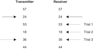
Both the receiver and the transmitter use a common algorithm to generate a pseudorandom sequence of addresses. This algorithm works by manipulating the address bits in a certain fashion. Thus, starting at a known address, both sides of the link will create the same next address. For demonstration purposes, Figure 4.13 shows the same sequence of two-digit decimal numbers at the transmitting side and the receiving side. The solid transmitter arrow points to the present transmitter address and the solid receiver arrow points to the expected receiver address. After transmission and reception, both transmitter and receiver calculate their next addresses, which will be the same. The arrows are synchronized to point to the same address during a system set-up procedure. As long as the receiver doesn't miss a transmission, there is no problem, since each side will calculate an identical next address. However, if one or more transmissions are missed by the receiver, when it finally does receive a message, its expected address will not match the received address. In this case it will perform its algorithm again to create a new address and will try to match it. If the addresses still don't match, a new address is calculated until either the addresses match or a given number of trials have been made with no success. At this point, the transmitter and receiver are unsynchronized and the original setup procedure has to be repeated to realign the transmitter and receiver addresses.

The number of trials permitted by the receiver may typically be between 64 and 256. If this number is too high, the possibility of compromising the system is greater (although with a 36-bit address a very large number of trials would be needed for this) and with too few trials, the frequency of inconvenient resynchronization would be greater. Note that a large number of trials takes a lot of time for computations and may cause a significant delay in response.

Several companies make rolling code components, among them Microchip, Texas Instruments, and National Semiconductor.

Data Field

The next part of the message frame is the data field. Its number of bits depends on how many pieces of information the transmitter may send to the receiver. For example, the motion detector may transmit three types of information: motion detection, tamper detection, or low battery.

Parity Bit Field

The last field is for error detection bits, or parity bits. As discussed later, some protocols have inherent error detection features so the last field is not needed.

Baseband Data Rate

Once we have determined the data frame, we can decide on the appropriate baseband data rate. For the security system example, this rate will usually be several hundred hertz up to a maximum of a couple of kilohertz. Since a rapid response is not needed, a frame can be repeated several times to be more certain it will get through. Frame repetition is needed in systems where space diversity is used in the receiver. In these systems, two separate antennas are periodically switched to improve the probability of reception. If signal nulling occurs at one antenna because of the multipath phenomena, the other antenna will produce a stronger signal, which can be correctly decoded. Thus, a message frame must be sent more often to give it a chance to be received after unsuccessful reception by one of the antennas.

Supervision

Another characteristic of digital event systems is the need for link supervision. Security systems and other event systems, including medical emergency systems, are one-way links. They consist of several transmitters and one receiver. As mentioned above, these systems transmit relatively rarely, only when there is an alarm or possibly a low-battery condition. If a transmitter ceases to operate, due to a component failure, for example, or if there is an abnormal continuing interference on the radio channel, the fact that the link has been broken will go undetected. In the case of a security system, the installation will be unprotected, possibly, until a routine system inspection is carried out. In a wired system, such a possibility is usually covered by a normally energized relay connected through closed contacts to a control panel. If a fault occurs in the device, the relay becomes unenergized and the panel detects the opening of the contacts. Similarly, cutting the connecting wires will also be detected by the panel. Thus, the advantages of a wireless system are compromised by the lower confidence level accompanying its operation.

Many security systems minimize the risk of undetected transmitter failure by sending a supervisory signal to the receiver at a regular interval. The receiver expects to receive a signal during this interval and can emit a supervisory alarm if the signal is not received. The supervisory signal must be identified as such by the receiver so as not to be mistaken for an alarm.

The duration of the supervisory interval is determined by several factors:

• Devices certified under FCC Part 15 paragraph 15.231, which applies to most wireless security devices in North America, may not send regular transmissions more frequently than one per hour.
• The more frequently regular supervision transmissions are made, the shorter the battery life of the device.
• Frequent supervisory transmissions when there are many transmitters in the system raise the probability of a collision with an alarm signal, which may cause the alarm not to get through to the receiver.
• The more frequent the supervisory transmissions, the higher the confidence level of the system.

While it is advantageous to notify the system operator at the earliest sign of transmitter malfunction, frequent supervision raises the possibility that a fault might be reported when it doesn't exist. Thus, most security systems determine that a number of consecutive missing supervisory transmissions must be detected before an alarm is given. A system which specifies security emissions once every hour, for example, may wait for eight missing supervisory transmissions, or eight hours, before a supervisory alarm is announced. Clearly, the greater the consequences of lack of alarm detection due to a transmitter failure, the shorter the supervision interval must be.

4.10.1.2. Continuous Digital Data

In other systems flowing digital data must be transmitted in real time and the original source data rate will determine the baseband data rate. This is the case in wireless LANs and wireless peripheral-connecting devices. The data is arranged in message frames, which contain fields needed for correct transportation of the data from one side to the other, in addition to the data itself.

An example of a frame used in synchronous data link control (SDLC) is shown in Figure 4.14. It consists of beginning and ending bytes that delimit the frame in the message, address and control fields, a data field of undefined length, and check bits or parity bits for letting the receiver check whether the frame was correctly received. If it is, the receiver sends a short acknowledgment and the transmitter can continue with the next frame. If no acknowledgment is received, the transmitter repeats the message again and again until it is received. This is called an ARQ (automatic repeat query) protocol. In high-noise environments, such as encountered on radio channels, the repeated transmissions can significantly slow down the message throughput.

Figure 4.14. Synchronous data link control frame

More common today is to use a forward error control (FEC) protocol. In this case, there is enough information in the parity bits to allow the receiver to correct a small number of errors in the message so that it will not have to request retransmission. Although more parity bits are needed for error correction than for error detection alone, the throughput is greatly increased when using FEC on noisy channels.

In all cases, we see that extra bits must be included in a message to insure proper transmission, and the consequently longer frames require a higher transmission rate than what would be needed for the source data alone. This message overhead must be considered in determining the required bit rate on the channel, the type of digital modulation, and consequently the bandwidth.

4.10.1.3. Analog Transmission

Analog transmission devices, such as wireless microphones, also have a baseband bandwidth determined by the data source. A high-quality wireless microphone may be required to pass 50 to 15,000 Hz, whereas an analog wireless telephone needs only 100 to 3000 Hz. In this case determining the channel bandwidth is more straightforward than in the digital case, although the bandwidth depends on whether AM or FM modulation is used. In most short-range radio applications, FM is preferred—narrow-band FM for voice communications and wide-band FM for quality voice and music transmission.

4.10.2. Baseband Coding

The form of the information signal that is modulated onto the RF carrier we call here baseband coding. We refer below to both digital and analog systems, although strictly speaking the analog signal is not coded but is modified to obtain desired system characteristics.

4.10.2.1. Digital Systems

Once we have a message frame, composed as we have shown by address and data fields, we must form the information into signal levels that can be effectively transmitted, received, and decoded. Since we're concerned here with binary data transmission, the baseband coding selected has to give the signal the best chance to be decoded after it has been modified by noise and the response of the circuit and channel elements. This coding consists essentially of the way that zeros and ones are represented in the signal sent to the modulator of the transmitter.

There are many different recognized systems of baseband coding. We will examine only a few common examples.

These are the dominant criteria for choosing or judging a baseband code:

• Timing. The receiver must be able to take a data stream polluted by noise and recognize transitions between each bit. The bit transitions must be independent of the message content—that is, they must be identifiable even for long strings of zeros or ones.
• DC content. It is desirable that the average level of the message—that is, its DC level—remains constant throughout the message frame, regardless of the content of the message. If this is not the case, the receiver detection circuits must have a frequency response down to DC so that the levels of the message bits won't tend to wander throughout the frame. In circuits where coupling capacitors are used, such a response is impossible.
• Power spectrum. Baseband coding systems have different frequency responses. A system with a narrow frequency response can be filtered more effectively to reduce noise before detection.
• Inherent error detection. Codes that allow the receiver to recognize an error on a bit-by-bit basis have a lower possibility of reporting a false alarm when error-detecting bits are not used.
• Probability of error. Codes differ in their ability to properly decode a signal, given a fixed transmitter power. This quality can also be stated as having a lower probability of error for a given signal-to-noise ratio.
• Polarity independence. There is sometimes an advantage in using a code that retains its characteristics and decoding capabilities when inverted. Certain types of modulation and demodulation do not retain polarity information. Phase modulation is an example.

Now let's look at some common codes (Figure 4.15) and rate them according to the criteria above. It should be noted that coding considerations for event-type reporting are far different from those for flowing real-time data, since bit or symbol times are not so critical, and message frames can be repeated for redundancy to improve the probability of detection and reduce false alarms. In data flow messages, the data rate is important and sophisticated error detection and correction techniques are used to improve system sensitivity and reliability.

• Non-return to Zero (NRZ)—Figure 4.15a.

Figure 4.15. Baseband bit formats

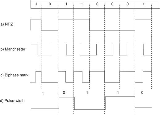
This is the most familiar code, since it is used in digital circuitry and serial wired short-distance communication links, like RS-232. However, it is rarely used directly for wireless communication. Strings of ones or zeros leave it without defined bit boundaries, and its DC level is very dependent on the message content. There is no inherent error detection. If NRZ coding is used, an error detection or correction field is imperative. If amplitude shift keying (ASK) modulation is used, a string of zeros means an extended period of no transmission at all. In any case, if NRZ signaling is used, it should only be for very short frames of no more than eight bits.

• Manchester code—Figure 4.15b.

A primary advantage of this code is its relatively low probability of error compared to other codes. It is the code used in Ethernet local area networks. It gives good timing information since there is always a transition in the middle of a bit, which is decoded as zero if this is a positive transition and a one otherwise. The Manchester code has a constant DC component and its waveform doesn't change if it passes through a capacitor or transformer. However, a “training” code sequence should be inserted before the message information as a preamble to allow capacitors in the receiver detection circuit to reach charge equilibrium before the actual message bits appear. Inverting the Manchester code turns zeros to ones and ones to zeros. The frequency response of Manchester code has components twice as high as NRZ code, so a low-pass filter in the receiver must have a cut-off frequency twice as high as for NRZ code with the same bit rate.

• Biphase Mark—Figure 4.15c.

This code is somewhat similar to the Manchester code, but bit identity is determined by whether or not there is a transition in the middle of a bit. For biphase mark, a level transition in the middle of a bit (going in either direction) signifies a one, and a lack of transition indicates zero. Biphase space is also used, where the space character has a level transition. There is always a transition at the bit boundaries, so timing content is good. A lack of this transition gives immediate notice of a bit error and the frame should then be aborted. The biphase code has constant DC level, no matter what the message content, and a preamble should be sent to allow capacitor charge equalization before the message bits arrive. As with the Manchester code, frequency content is twice as much as for the NRZ code. The biphase mark or space code has the added advantage of being polarity independent.

• Pulse width modulation—Figure 4.15d.

As shown in the figure, a one has two timing durations and a zero has a pulse width of one duration. The signal level inverts with each bit so timing information for synchronization is good. There is a constant average DC level. Since the average pulse width varies with the message content, in contrast with the other examples, the bit rate is not constant. This code has inherent error detection capability.

• Motorola MC145026-145028 coding—Figure 4.16.

  Figure 4.16. Motorola MC145026

  

Knowledge of the various baseband codes is particularly important if the designer creates his own protocol and implements it on a microcontroller. However, there are several off-the-shelf integrated circuits that are popular for simple event transmission transmitters where a microcontroller is not needed for other circuit functions, such as in panic buttons or door-opening controllers.

The Motorola chips are an example of nonstandard coding developed especially for event transmission where three-state addressing is determined as high, low, or open connections to device pins. Thus, a bit symbol can be one of three different types. The receiver, MC145028, must recognize two consecutive identical frames to signal a valid message. The Motorola protocol gives very high reliability and freedom from false alarms. Its signal does have a broad frequency spectrum relative to the data rate and the receiver filter passband must be designed accordingly. The DC level is dependent on the message content.

4.10.2.2. Analog Baseband Conditioning

Wireless microphones and headsets are examples of short-range systems that must maintain high audio quality over the vagaries of changing path lengths and indoor environments, while having small size and low cost. To help them achieve this, they have a signal conditioning element in their baseband path before modulation. Two features used to achieve high signal-to-noise ratio over a wide dynamic range are pre-emphasis/de-emphasis and compression/expansion. Their positions in the transmitter/receiver chain are shown in Figure 4.17.

Figure 4.17. Wireless microphone system

The transmitter audio signal is applied to a high-pass filter (pre-emphasis) which increases the high frequency content of the signal. In the receiver, the detected audio goes through a complementary low-pass filter (de-emphasis), restoring the signal to its original spectrum composition. However, in so doing, high frequency noise that entered the signal path after the modulation process is filtered out by the receiver while the desired signal is returned to its original quality.

Compression of the transmitted signal raises the weak sounds and suppresses strong sounds to make the modulation more efficient. Reversing the process in the receiver weakens annoying background noises while restoring the signal to its original dynamic range.

4.10.3. RF Frequency and Bandwidth

There are several important factors to consider when determining the radio frequency of a short-range system:

• Telecommunication regulations
• Antenna size
• Cost
• Interference
• Propagation characteristics

When you want to market a device in several countries and regions of the world, you may want to choose a frequency that can be used in the different regions, or at least frequencies that don't differ very much so that the basic design won't be changed by changing frequencies.

The UHF frequency bands are usually the choice for wireless alarm, medical, and control systems. The bands that allow unlicensed operation don't require rigid frequency accuracy. Various components—SAWs and ICs—have been specially designed for these bands and are available at low prices, so choosing these frequencies means simple designs and low cost. Many companies produce complete RF transmitter and receiver modules covering the most common UHF frequencies, among them 315 MHz and 902 to 928 MHz (U.S. and Canada), and 433.92 MHz band and 868 to 870 MHz (European Community).

Antenna size may be important in certain applications, and for a given type of antenna, its size is proportional to wavelength, or inversely proportional to frequency. When spatial diversity is used to counter multipath interference, a short wavelength of the order of the size of the device allows using two antennas with enough spacing to counter the nulling that results from multipath reflections. In general, efficient built-in antennas are easier to achieve in small devices at short wavelengths.

From VHF frequencies and up, cost is directly proportional to increased frequency.

Natural and manmade background noise is higher on the lower frequencies. On the other hand, certain frequency bands available for short-range use may be very congested with other users, such as the ISM bands. Where possible, it is advisable to chose a band set aside for a particular use, such as the 868–870 MHz band available in Europe.

Propagation characteristics also must be considered in choosing the operating frequency. High frequencies reflect easily from surfaces but penetrate insulators less readily than lower frequencies.

The radio frequency bandwidth is a function of the baseband bandwidth and the type of modulation employed. For security event transmitters, the required bandwidth is small, of the order of several kilohertz. If the complete communication system were designed to take advantage of this narrow bandwidth, there would be significant performance advantages over the most commonly used systems having a bandwidth of hundreds of kilohertz. For given radiated transmitter power, the range is inversely dependent on the receiver bandwidth. Also, narrow-band unlicensed frequency allotments can be used where available in the different regions, reducing interference from other users. However, cost and complexity considerations tend to outweigh communication reliability for these systems, and manufacturers decide to make do with the necessary performance compromises. The bandwidth of the mass production security devices is thus determined by the frequency stability of the transmitter and receiver frequency determining elements, and not by the required signaling bandwidth. The commonly used SAW devices dictate a bandwidth of at least 200 kHz, whereas the signaling bandwidth may be only 2 kHz. Designing the receiver with a passband of 20 kHz instead of 200 kHz would increase sensitivity by 10 dB, roughly doubling the range. This entails using stable crystal oscillators in the transmitter and in the receiver local oscillator.

4.10.4. Modulation

Amplitude modulation (AM) and frequency modulation (FM), known from commercial broadcasting, have their counterparts in modulation of digital signals, but you must be careful before drawing similar conclusions about the merits of each. The third class of modulation is phase modulation, not used in broadcasting, but its digital counterpart is commonly used in high-end, high-data-rate digital wireless communication.

Digital AM is referred to as ASK—amplitude shift keying—and sometimes as OOK—on/off keying. FSK is frequency shift keying, the parallel to FM. Commercial AM has a bandwidth of 10 kHz whereas an FM broadcasting signal occupies 180 kHz. The high post-detection signal-to-noise ratio of FM is due to this wide bandwidth. However, on the negative side, FM has what is called a threshold effect, also due to wide bandwidth. Weak FM signals are unintelligible at a level that would still be usable for AM signals. When FM is used for two-way analog communication, narrow-band FM, which occupies a similar bandwidth to AM, also has comparable sensitivity for a given S/N.

4.10.4.1. Modulation for Digital Event Communication

For short-range digital communication we're not interested in high fidelity, but rather high sensitivity. Other factors for consideration are simplicity and cost of modulation and demodulation. Let's now look into the reasons for choosing one form of modulation or the other.

An analysis of error rates versus bit energy to noise density shows that there is no inherent advantage of one system, ASK or FSK, over the other. This conclusion is based on certain theoretical assumptions concerning bandwidth and method of detection. While practical implementation methods may favor one system over the other, we shouldn't jump to conclusions that FSK is necessarily the best, based on a false analogy to FM and AM broadcasting.

In low-cost security systems, ASK is the simplest and cheapest method to use. For this type of modulation we must just turn on and turn off the radio frequency output in accordance with the digital modulating signal. The output of a microcontroller or dedicated coding device biases on and off a single SAW-controlled transistor RF oscillator. Detection in the receiver is also simple. It may be accomplished by a diode detector in several receiver architectures, to be discussed later, or by the RSSI (received signal strength indicator) output of many superheterodyne receiver ICs employed today. Also, ASK must be used in the still widespread superregenerative receivers.

For FSK, on the other hand, it's necessary to shift the transmitting frequency between two different values in response to the digital code. More elaborate means is needed for this than in the simple ASK transmitter, particularly when crystal or SAW devices are used to keep the frequency stable. In the receiver, also, additional components are required for FSK demodulation as compared to ASK. We have to decide whether the additional cost and complexity is worthwhile for FSK.

In judging two systems of modulation, we must base our results on a common parameter that is a basis for comparison. This may be peak or average power. For FSK, the peak and average powers are the same. For ASK, average power for a given peak power depends on the duty cycle of the modulating signal. Let's assume first that both methods, ASK and FSK, give the same performance—that is, the same sensitivity—if the average power in both cases are equal. It turns out that in this case, our preference depends on whether we are primarily marketing our system in North America or in Europe. This is because of the difference in the definition of the power output limits between the telecommunication regulations in force in the US and Canada as compared to the common European regulations.

The US FCC Part 15 and similar Canadian regulations specify an average field strength limit. Thus, if the transmitter is capable of using a peak power proportional to the inverse of its modulation duty cycle, while maintaining the allowed average power, then under our presumption of equal performance for equal average power, there would be no reason to prefer FSK, with its additional complexity and cost, over ASK.

In Western Europe, on the other hand, the low-power radio specification, ETSI 300 220limits the peak power of the transmitter. This means that if we take advantage of the maximum allowed peak power, FSK is the proper choice, since for a given peak power, the average power of the ASK transmitter will always be less, in proportion to the modulating signal duty cycle, than that of the FSK transmitter.

However, is our presumption of equal performance for equal average power correct? Under conditions of added white Gaussian noise (AWGN) it seems that it is. This type of noise is usually used in performance calculations since it represents the noise present in all electrical circuits as well as cosmic background noise on the radio channel. But in real life, other forms of interference are present in the receiver passband that have very different, and usually unknown, statistical characteristics from AWGN. On the UHF frequencies normally used for short-range radio, this interference is primarily from other transmitters using the same or nearby frequencies. To compare performance, we must examine how the ASK and FSK receivers handle this type of interference. This examination is pertinent in the US and Canada where we must choose between ASK and FSK when considering that the average power, or signal-to-noise ratio, remains constant. Some designers believe that a small duty cycle resulting in high peak power per bit is advantageous since the presence of the bit, or high peak signal, will get through a background of interfering signals better than another signal with the same average power but a lower peak. To check this out, we must assume a fair and equal basis of comparison. For a given data rate, the low-duty-cycle ASK signal will have shorter pulses than for the FSK case. Shorter pulses means higher baseband bandwidth and a higher cutoff frequency for the post detection bandpass filter, resulting in more broadband noise for the same data rate. Thus, the decision depends on the assumptions of the type of interference to be encountered and even then the answer is not clear cut.

An analysis of the effect of different types of interference is given by Anthes of RF Monolithics (see references). He concludes that ASK, which does not completely shut off the carrier on a “0” bit, is marginally better than FSK.

4.10.4.2. Continuous Digital Communication

For efficient transmission of continuous digital data, the modulation choices are much more varied than in the case of event transmission. We can see this in the three leading cellular digital radio systems, all of which have the same use and basic requirements. The system referred to as DAMPS or TDMA (time division multiple access) uses a type of modulation called Pi/4 DPSK (differential phase shift keying). The GSM network is based on GMSK (Gaussian minimum shift keying). The third major system is CDMA (code division multiple access). Each system claims that its choice is best, but it is clear that there is no simple cut-and-dried answer. We aren't going into the details of the cellular systems here, so we'll look at the relevant trade-offs for modulation methods in what we have defined as short-range radio applications. At the end of this section, we review the basic principles of digital modulation and spread-spectrum modulation.

For the most part, license-free applications specify ISM bands where signals are not confined to narrow bandwidth channels. However, noise power is directly proportional to bandwidth, so the receiver bandwidth should be no more than is required for the data rate used. Given a data rate and an average or peak power limitation, there are several reasons for preferring one type of modulation over another. They involve error rate, implementation complexity, and cost. A common way to compare performance of the different systems is by curves of bit error rate (BER) versus the signal-to-noise ratio, expressed as energy per bit divided by the noise density (defined below). The three most common types of modulation system are compared in Figure 4.18. Two of the modulation types were mentioned above. The third, phase shift keying, is described below.

Figure 4.18. Bit error rates

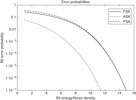
Phase Shift Keying (PSK)

Whereas in amplitude shift keying and frequency shift keying the amplitude and frequency are varied according to the digital source data, in PSK it is the phase of the RF carrier that is varied. In its simplest form, the waveform looks like Figure 4.19. Note that the phase of the carrier wave shifts 180 deg. according to the data signal bits. Similar to FSK, the carrier remains constant, thus giving the same advantage that we mentioned for FSK—maximum signal-to-noise ratio when there is a peak power limitation.

Figure 4.19. Phase shift keying

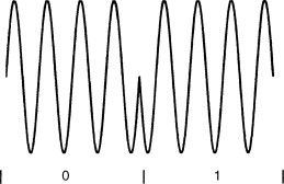
Comparing Digital Modulation Methods

In comparing the different digital modulation methods, we need a common reference parameter that reflects the signal power and noise at the input of the receiver, and the bit rate of the data. This common parameter of signal to noise ratio for digital systems is expressed as the signal energy per bit divided by the noise density, E/N^o. We can relate this parameter to the more familiar signal to noise ratio, S/N, and the data rate R, as follows:

1. S/N=signal power/noise power. The noise power is the noise density N^o in watts/Hz times the transmitted signal bandwidth B^T in Hz:

2. The signal energy in joules is the signal power in watts, S, times the bit time in seconds, which is 1/(data rate)=1/R, thus E=S(1/R)

3. The minimum transmitted bandwidth (Nyquist bandwidth) to pass a bit stream of R bits per second is B^T=R Hz.

4. In sum:

The signal power for this expression is the power at the input of the receiver, which is derived from the radiated transmitted power, the receiver antenna gain, and the path loss. The noise density N^o, or more precisely the one sided noise power spectral density, in units of watts/Hz, can be calculated from the expression:

The factor k is Boltzmann's constant and T is the equivalent noise temperature that relates the receiver input noise to the thermal noise that is present in a resistance at the same temperature T. Thus, at standard room temperature of 290 degrees Kelvin, the noise power density is 4×10⁻²¹ watts/Hz, or −174 dBm/Hz.

The modulation types making up the curves in Figure 4.18 are:

Phase shift keying (PSK)

Noncoherent frequency shift keying (FSK)

Noncoherent amplitude shift keying (ASK)

We see from the curves that the best type of modulation to use from the point of view of lowest bit error for a given signal-to-noise ratio (E/N^o) is PSK. There is essentially no difference, according to the curves, between ASK and FSK. (This is true only when noncoherent demodulation is used, as in most simple short-range systems.) What then must we consider in making our choice?

PSK is not difficult to generate. It can be done by a balanced modulator. The difficulty is in the receiver. A balanced modulator can be used here too but one of its inputs, which switches the polarity of the incoming signal, must be perfectly correlated with the received signal carrier and without its modulation. The balanced modulator acts as a multiplier and when a perfectly synchronized RF carrier is multiplied by the received signal, the output, after low-pass filtering, is the original bit stream. PSK demodulation is shown in Figure 4.20.

Figure 4.20. PSK demodulation

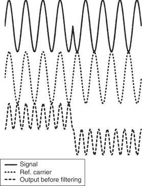
There are several ways of generating the required reference carrier signal from the received signal. Two examples are the Costas loop and the squaring loop, which include three multiplier blocks and a variable frequency oscillator (VFO). [See Dixon.] Because of the complexity and cost, PSK is not commonly used in inexpensive short-range equipment, but it is the most efficient type of modulation for high-performance data communication systems.

Amplitude shift keying is easy to generate and detect, and as we see from Figure 4.18, its bit error rate performance is essentially the same as for FSK. However, FSK is usually the modulation of choice for many systems. The primary reason is that peak power is usually the limitation, which gives FSK a 3-dB advantage, since it has constant power for both bit states, whereas ASK has only half the average power, assuming a 50% duty cycle and equal probability of marks and spaces. FSK has slightly more complexity than ASK, and that's probably why it isn't used in all short-range digital systems.

A modulation system which incorporates the methods discussed above but provides a high degree of interference immunity is spread spectrum, which we'll discuss later on in this chapter.

4.10.4.3. Analog Communication

For short-range analog communication—wireless microphones, wireless earphones, auditive assistance devices—FM is almost exclusively used. When transmitting high-quality audio, FM gives an enhanced post-detection signal-to-noise ratio, at the expense of greater bandwidth. Even for narrow band FM, which doesn't have post-detection signal-to-noise enhancement, its noise performance is better than that of AM, because a limiting IF amplifier can be used to reduce the noise. AM, being a linear modulation process, requires linear amplifiers after modulation in the transmitter, which are less efficient than the class C amplifiers used for FM. Higher power conversion efficiency gives FM an advantage in battery-operated equipment.

4.10.4.4. Advanced Digital Modulation

Two leading characteristics of wireless communication in the last few years are the need for increasing data rates and better utilization of the radio spectrum. This translates to higher speeds on narrower bandwidths. At the same time, much of the radio equipment is portable and operated by batteries. So what is needed is:

• high data transmission rates
• narrow bandwidth
• low error rates at low signal-to-noise ratios
• low power consumption

Breakthroughs have occurred with the advancement of digital modulation and coding systems. We deal here with digital modulation principles.

The types of modulation that we discussed previously, ASK, FSK, and PSK, involve modifying a radio frequency carrier one bit at a time. We mentioned the Nyquist bandwidth, which is the narrowest bandwidth of an ideal filter which permits passing a bit stream without intersymbol interference. As the bandwidth of the digital bit stream is further reduced, the bits are lengthened and interfere with the detection of subsequent bits. This minimum, or Nyquist, bandwidth equals one-half of the bit rate at baseband, but twice as much for the modulated signal. We can see this result in Figure 4.21. An alternating series of marks and spaces can be represented by a sine wave whose frequency is one-half the bit rate: f^sin=1/2T. An ideal filter with a lower cutoff frequency will not pass this fundamental frequency component and the data will not get through.

Figure 4.21. Nyquist bandwidth

Any other combination of bits will create other frequencies, all of which are lower than the Nyquist frequency. It turns out then that the maximum number of bits per hertz of filter cutoff frequency that can be passed at baseband is two. Therefore, if the bandwidth of a telephone line is 3.4 kHz, the maximum binary bit rate that it can pass without intersymbol interference is 6.8k bits per second. We know that telephone line modems pass several times this rate. They do it by incorporating several bits in each symbol transmitted, for it is actually the symbol rate that is limited by the Nyquist bandwidth, and the problem that remains is to put several bits on each symbol in such a manner that they can be effectively taken off the symbol at the receiving end with as small as possible chance of error, given a particular S/N.

In Figure 4.22 we see three ways of combining bits with individual symbols, each of them based on one of the basic types of modulation—ASK, FSK, PSK. Each symbol duration T can carry one of four different values, or two bits. Using any one of the modulation types shown, the telephone line, or wireless link, can pass a bit rate twice as high as before over the same bandwidth. Combinations of these types are also employed, particularly of ASK and PSK, to put even more bits on a symbol. Quadrature amplitude modulation, QAM, sends several signal levels on four phases of the carrier frequency to give a high bandwidth efficiency—a high bit-rate relative to the signal bandwidth. It seems then that there is essentially no limit to the number of bits that could be compressed into a given bandwidth. If that were true, the 3.4-kHz telephone line could carry millions of bits per second, and the internet bottleneck to our homes would no longer exist. However, there is a very definite limit to the rate of information transfer over a transmission medium where noise is present, expressed in the Hartley-Shannon law:

Figure 4.22. M-ary modulation

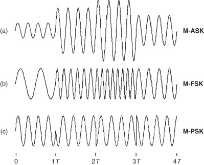
This expression tells us that the maximum rate of information (the capacity C) that can be sent without errors on a communication link is a function of the bandwidth, W, and the signal-to-noise ratio, S/N.

In investigating the ways of modulating and demodulating multiple bits per symbol, we'll first briefly discuss a method not commonly used in short-range applications (although it could be). This is called M-ary FSK (Figure 4.22b) and in contrast to the aim we mentioned above of increasing the number of bits per hertz, it increases the required bandwidth as the number of bits per symbol is increased. “M” in “M-FSK” is the number of different frequencies that may be transmitted in each symbol period. The benefit of this method is that the required S/N per bit for a given bit error rate decreases as the number of bits per symbol increases. This is analogous to analog FM modulation, which uses a wideband radio channel, well in excess of the bandwidth of the source audio signal, to increase the resultant S/N. M-ary FSK is commonly used in point-to-point microwave transmission links for high-speed data communication where bandwidth limitation is no problem but the power limitation is.

Most of the high-data-rate bandwidth-limited channels use multiphase PSK or QAM. While there are various modulation schemes in use, the essentials of most of them can be described by the block diagram in Figure 4.23. This diagram is the basis of what may be called vector modulation, IQ modulation, or quadrature modulation. “I” stands for “in phase” and “Q” stands for “quadrature.”

Figure 4.23. Quadrature modulation

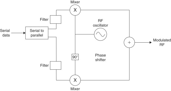
The basis for quadrature modulation is the fact that two completely independent data streams can be simultaneously modulated on the same frequency and carrier wave. This is possible if each data stream modulates coherent carriers whose phases are 90 degrees apart. We see in the diagram that each of these carriers is created from the same source by passing one of them through a 90-degree phase shifter. Now it doesn't matter which method of modulation is used for each of the phase shifted carriers. Although the two carriers are added together and amplified before transmission, the receiver, by reversing the process used in the transmitter (see Figure 4.24), can completely separate the incoming signal into its two components.

Figure 4.24. Quadrature demodulation

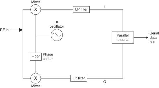
The diagrams in Figures 4.23 and 4.24 demonstrate quadrature phase shift keying (QPSK) where a data stream is split into two, modulated independently bit by bit, then combined to be transmitted on a single carrier. The receiver separates the two data streams, then demodulates and combines them to get the original serial digital data. The phase changes of the carrier in response to the modulation is commonly shown on a vector or constellation diagram. The constellation diagram for QPSK is shown in Figure 4.25. The Xs on the plot are tips of vectors that represent the magnitude (distance from the origin) and phase of the signal that is the sum of the “I” and the “Q” carriers shown on Figure 4.23, where each is multiplied by −1 or +1, corresponding to bit values of 0 and 1. The signal magnitudes of all four possible combinations of the two bits are the same—

when the I and Q carriers have a magnitude of 1. I and Q bit value combinations corresponding to each vector are shown on the plot.

Figure 4.25. QPSK constellation diagram

We have shown that two data streams, derived from a data stream of rate R2, can be sent in parallel on the same RF channel and at the same bandwidth as a single data stream having half the bit rate, R1. At the receiver end, the demodulation process of each of the split bit streams is exactly the same as it would be for the binary phase shift modulation shown in Figure 4.20 above, and its error rate performance is the same as is shown for the BPSK curve in Figure 4.18. Thus, we've doubled the data rate on the same bandwidth channel while maintaining the same error rate as before. In short, we've doubled the efficiency of the communication.

However, there are some complications in adopting quadrature modulation. Similar to the basic modulation methods previously discussed, the use of square waves to modulate RF carriers causes unwanted sidebands that may exceed the allowed channel bandwidth. Thus, special low-pass filters, shown in Figure 4.23, are inserted in the signal paths before modulation. Even with these filters, the abrupt change in the phase of the RF signal at the change of data state will also cause increased sidebands. We can realize from Figure 4.22c that changes of data states may cause the RF carrier to pass through zero when changing phase. Variations of carrier amplitude make the signal resemble amplitude modulation, which requires inefficient linear amplifiers, as compared to nonlinear amplifiers that can be used for frequency modulation, for example.

Two variations of quadrature phase shift keying have been devised to reduce phase changes between successive symbols and to prevent the carrier from going through zero amplitude during phase transitions. One of these is offset phase shift keying. In this method, the I and Q data streams in the transmitter are offset in time by one-half of the bit duration, causing the carrier phase to change more often but more gradually. In other words, the new “I” bit will modulate the cosine carrier at half a bit time earlier (or later) than the time that the “Q” bit modulates the sine carrier.

The other variant of QPSK is called pi/4 DPSK. It is used in the US TDMA (time division multiple access) digital cellular system. In it, the constellation diagram is rotated pi/4 radians (45 degrees) at every bit time such that the carrier phase angle can change by either 45 or 135 degrees. This system reduces variations of carrier amplitude so that more efficient nonlinear power amplifiers may be used in the transmitter.

Another problem with quadrature modulation as described above is the need for a coherent local oscillator in the receiver in order to separate the in-phase and quadrature data streams. As for bipolar phase shift keying, this problem may be ameliorated by using differential modulation and by multiplying a delayed replica of the received signal by itself to extract the phase differences from symbol to symbol.

The principle of transmitting separate data streams on in phase and quadrature RF carriers may be extended so that each symbol on each carrier contains 2, 3, 4 or more bits. For example, 4 bits per each carrier vector symbol allows up to 16 amplitude levels per carrier and a total of 256 different states of amplitude and phase altogether. This type of modulation is called quadrature amplitude modulation (QAM), and in this example, 256-QAM, 8 data bits can be transmitted in essentially the same time and bandwidth as one bit sent by binary phase shift keying. The constellation of 16-QAM (4 bits per symbol) is shown in Figure 4.26.

Figure 4.26. 16-QAM constellation diagram

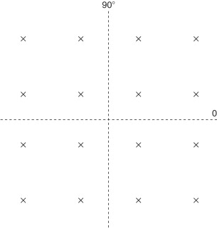
Remember that the process of concentrating more and more bits to a carrier symbol cannot go on without limit. While the bit rate per hertz goes up, the required S/N of the channel for a given bit error rate (BER) also increases—that is, more power must be transmitted, or as a common alternative in modern digital communication systems, sophisticated coding algorithms are incorporated in the data protocol. However, the ultimate limit of data rate for a particular communication channel with noise is the Hartley-Shannon limit stated above.

We now turn to examine another form of digital modulation that is becoming very important in a growing number of short-range wireless applications—spread-spectrum modulation.

4.10.4.5. Spread Spectrum

The regulations for unlicensed communication using unspecified modulation schemes, both in the US and in Europe, determine maximum power outputs ranging from tens of microwatts up to 10 milliwatts in most countries. This limitation greatly reduces the possibilities for wireless devices to replace wires and to obtain equivalent communication reliability. However, the availability of frequency bands where up to one watt may be transmitted in the US and 100 mW in Europe, under the condition of using a specified modulation system, greatly enlarges the possible scope of use and reliability of unlicensed short-range communication.

Spread spectrum has allowed the telecommunication authorities to permit higher transmitter powers because spread-spectrum signals can coexist on the same frequency bands as other types of authorized transmissions without causing undue interference or being unreasonably interfered with. The reason for this is evident from Figure 4.27. Figure 4.27a shows the spread-spectrum signal spread out over a bandwidth much larger than the narrow-band signals. Although its total power if transmitted as a narrow band signal could completely overwhelm another narrow-band signal on the same or adjacent frequency, the part of it occupying the narrow-band signal bandwidth is small related to the total, so it doesn't interfere with it. In other words, spreading the transmitted power over a wide frequency band greatly reduces the signal power in a narrow bandwidth and thus the potential for interference.

Figure 4.27. Spread spectrum and narrow-band signals

Figure 4.27b shows how spread-spectrum processing reduces interference from adjacent signals. The de-spreading process concentrates the total power of the spread-spectrum signal into a narrow-band high peak power signal, whereas the potentially interfering narrow-band signals are spread out so that their power in the bandwidth of the desired signal is relatively low.

These are some advantages of spread spectrum modulation:

• FCC rules allow higher power for nonlicensed devices
• Reduces co-channel interference—good for congested ISM bands
• Reduces multipath interference
• Resists intentional and unintentional jamming
• Reduces the potential for eavesdropping
• Permits code division multiplexing of multiple users on a common channel.

There is sometimes a tendency to compare spread spectrum with wide-band frequency modulation, such as used in broadcasting, since both processes achieve performance advantages by occupying a channel bandwidth much larger than the bandwidth of the information being transmitted. However, it's important to understand that there are principal differences in the two systems.

In wide band FM (WBFM), the bandwidth is spread out directly by the amplitude of the modulating signal and at a rate determined by its frequency content. The result achieved is a signal-to-noise ratio that is higher than that obtainable by sending the same signal over baseband (without modulation) and with the same noise density as on the RF channel. In WBFM, the post detection signal-to-noise ratio (S/N) is a multiple of the S/N at the input to the receiver, but that input S/N must be higher than a threshold value, which depends on the deviation factor of the modulation.

In contrast, spread spectrum has no advantage over baseband transmission from the point of view of signal-to-noise ratio. Usual comparisons of modulation methods are based on a channel having only additive wideband Gaussian noise. With such a basis for comparison, there would be no advantage at all in using spread spectrum compared to sending the same data over a narrow-band link. The advantages of spread spectrum are related to its relative immunity to interfering signals, to the difficulty of message interception by a chance eavesdropper, and to its ability to use code selective signal differentiation. Another often-stated advantage to spread spectrum—reduction of multipath interference—is not particularly relevant to short-range communication because the pulse widths involved are much longer than the delay times encountered indoors. (A spread-spectrum specialist company, Digital Wireless, claims a method of countering multipath interference over short distances.)

The basic difference between WBFM and spread spectrum is that the spreading process of the latter is completely independent of the baseband signal itself. The transmitted signal is spread by one (or more) of several different spreading methods, and then un-spread in a receiver that knows the spreading code of the transmitter.

The methods for spreading the bandwidth of the spread-spectrum transmission are frequency-hopping spread spectrum (FHSS), direct-sequence spread spectrum (DSSS), pulsed-frequency modulation or chirp modulation, and time-hopping spread spectrum. The last two types are not allowed in the FCC rules for unlicensed operation and after giving a brief definition of them we will not consider them further.

1. In frequency-hopping spread spectrum, the RF carrier frequency is changed relatively rapidly at a rate of the same order of magnitude as the bandwidth of the source information (analog or digital), but not dependent on it in any way. At least several tens of different frequencies are used, and they are changed according to a pseudo-random pattern known also at the receiver. The spectrum bandwidth is roughly the number of the different carrier frequencies times the bandwidth occupied by the modulation information on one hopping frequency.

2. The direct-sequence spread-spectrum signal is modulated by a pseudo-random digital code sequence known to the receiver. The bit rate of this code is much higher than the bit rate of the information data, so the bandwidth of the RF signal is consequently higher than the bandwidth of the data.

3. In chirp modulation, the transmitted frequency is swept for a given duration from one value to another. The receiver knows the starting frequency and duration so it can unspread the signal.

4. A time-hopping spread-spectrum transmitter sends low duty cycle pulses with pseudo-random intervals between them. The receiver unspreads the signal by gating its reception path according to the same random code as used in the transmitter.

Actually, all of the above methods, and their combinations that are sometimes employed, are similar in that a pseudo-random or arbitrary (in the case of chirp) modulation process used in the transmitter is duplicated in reverse in the receiver to unravel the wide-band transmission and bring it to a form where the desired signal can be demodulated like any narrowband transmission.

The performance of all types of spread-spectrum signals is strongly related to a property called process gain. It is this process gain that quantifies the degree of selection of the desired signal over interfering narrow-band and other wide-band signals in the same passband. Process gain is the difference in dB between the output S/N after unspreading and the input S/N to the receiver:

The process gain factor may be approximated by the ratio

A possibly more useful indication of the effectiveness of a spread-spectrum system is the jamming margin:

where L^sys is system implementation losses, which may be of the order of 2 dB.

The jamming margin is the amount by which a potentially interfering signal in the receiver's passband may be stronger than the desired signal without impairing the desired signal's ability to get through.

Let's now look at the details of frequency hopping and direct-sequence spread spectrum.

Frequency Hopping

FHSS can be divided into two classes—fast hopping and slow hopping. A fast-hopping transmission changes frequency one or more times per data bit. In slow hopping, several bits are sent per hopping frequency. Slow hopping is used for fast data rates since the frequency synthesizers in the transmitter and receiver are not able to switch and settle to new frequencies fast enough to keep up with the data rate if one or fewer bits per hop are transmitted. The spectrum of a frequency-hopping signal looks like Figure 4.28.

Figure 4.28. Spectrum of frequency-hopping spread spectrum signal

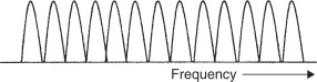
Figure 4.29 is a block diagram of FHSS transmitter and receiver. Both transmitter and receiver local oscillator frequencies are controlled by frequency synthesizers. The receiver must detect the beginning of a transmission and synchronize its synthesizer to that of the transmitter. When the receiver knows the pseudo-random pattern of the transmitter, it can lock onto the incoming signal and must then remain in synchronization by changing frequencies at the same time as the transmitter. Once exact synchronization has been obtained, the IF frequency will be constant and the signal can be demodulated just as in a normal narrow-band superheterodyne receiver. If one or more of the frequencies that the transmission occupies momentarily is also occupied by an interfering signal, the bit or bits that were transmitted at that time may be lost. Thus, the transmitted message must contain redundancy or error correction coding so that the lost bits can be reconstructed.

Figure 4.29. FHSS transmitter and receiver

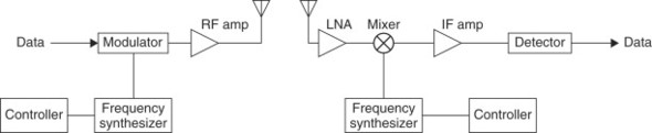
Direct Sequence

Figure 4.30 is a diagram of a DSSS system. A pseudo-random spreading code modulates the transmitter carrier frequency, which is then modulated by the data. The elements of this code are called chips. The frequency spectrum created is shown in Figure 4.31. The required bandwidth is the width of the major lobe, shown on the drawing as 2×Rc, or twice the chip rate. Due to the wide bandwidth, the signal-to-noise ratio at the receiver input is very low, often below 0 dB. The receiver multiplies a replica of the transmitter pseudo-random spreading code with the receiver local oscillator and the result is mixed with the incoming signal. When the transmitter and receiver spreading codes are the same and are in phase, a narrow-band IF signal results that can be demodulated in a conventional fashion.

Figure 4.30. DSSS transmitter and receiver

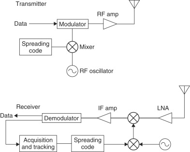
Figure 4.31. DSSS frequency spectrum

There are two stages to synchronizing transmitter and receiver pseudorandom codes—acquisition and tracking. In order to acquire a signal, the receiver multiplies the known expected code with the incoming RF signal. The output of this multiplication will be random noise when signals other than the desired signal exist on the channel. When the desired signal is present, it must be synchronized precisely in phase with the receiver's code sequence to achieve a strong output. A common way to obtain this synchronization is for the receiver to adjust its code to a rate slightly different from that of the transmitter. Then the phase difference between the two codes will change steadily until they are within one bit of each other, at which time the output of the multiplier increases to a peak when the codes are perfectly synchronized. This method of acquisition is called a sliding correlator.

The next stage in synchronization, tracking, keeps the transmitted and received code bits aligned for the complete duration of the message. In the method called “tau delta” the receiver code rate is varied slightly around the transmitted rate to produce an error signal that is used to create an average rate exactly equal to the transmitter's.

Other methods for code acquisition and tracking can be found in any book on spread spectrum—for example, Dixon's—listed in the references. Once synchronization has been achieved, the resulting narrow-band IF signal has a S/N equal to the received S/N plus the process gain, and it can be demodulated as any narrow-band signal. The difference in using spread spectrum is that interfering signals that would render the normal narrowband signal unintelligible are now reduced by the amount of the process gain.

Relative Advantages of DSSS and FHSS

The advantages of one method over the other are often debated, but there is no universally agreed-upon conclusion as to which is better, and both types are commonly used. They both are referenced in the IEEE specification 802.11 for wireless LANs. However some conclusions, possibly debatable, can be made:

• For a given data rate and output power, an FHSS system can be designed with less power consumption than DSSS.
• DSSS can provide higher data rates with less redundancy.
• Acquisition time is generally lower with FHSS (although short times are achieved with DSSS using matched filter and short code sequence).
• FHSS may have higher interference immunity, particularly when compared with DSSS with lowest allowed process gain.
• DSSS has more flexibility—frequency agility may be used to increase interference immunity.

4.10.5. RFID

A growing class of applications for short-range wireless is radio frequency identification (RFID). A basic difference between RFID and the applications discussed above is that RFID devices are not communication devices per se but involve interrogated transponders. Instead of having two separate transmitter and receiver terminals, an RFID system consists of a reader that sends a signal to a passive or active tag and then receives and interprets a modified signal reflected or retransmitted back to it.

The reader has a conventional transmitter and receiver having similar characteristics to the devices already discussed. The tag itself is special for this class of applications. It may be passive, receiving its power for retransmission from the signal sent from the reader, or it may have an active receiver and transmitter and tiny embedded long-life battery. Ranges of RFID may be several centimeters up to tens of meter. Operation frequencies range from 125 kHz up to 2.45 GHz. Frequencies are usually those specified for nonlicensed applications. Higher data rates demand higher frequencies.

In its most common form of operation, an RFID system works as follows. The reader transmits an interrogation signal, which is received by the tag. The tag may alter the incoming signal in some unique manner and reflect it back, or its transmitting circuit may be triggered to read its ID code residing in memory and to transmit this code back to the receiver. Active tags have greater range than passive tags. If the tag is moving in relation to the receiver, such as in the case of toll collection on a highway, the data transfer must take place fast enough to be complete before the tag is out of range.

These are some design issues for RFID:

• Tag orientation is likely to be random, so tag and reader antennas must be designed to give the required range for any orientation.
• Multiple tags within the transmission range can cause return message collisions. One way to avoid this is by giving the tags random delay times for response, which may allow several tags to be interrogated at once.
• Tags must be elaborately coded to prevent misreading.

4.11. Summary

This chapter has looked at various factors that affect the range of reliable wireless communication. Propagation of electromagnetic waves is influenced by physical objects in and near the path of line-of-sight between transmitter and receiver. We can get a first rough approximation of communication distance by considering only the reflection of the transmitted signal from the earth. We described several techniques of diversity reception that can reduce the required power for a given reliability when the communication link is subject to fading.

Noise was presented as the ultimate limitation on communication range. We saw that noise sources to be contended with depend on the operating frequency. The importance of low-noise receiver design depends on the relative intensity of noise received by the antenna to the noise generated in the receiver.

In this chapter we also examined various characteristics of short-range systems. We looked at the ways in which data is formatted into different information fields for transmission over a wireless link. We looked at several methods of encoding the one's and zero's of the baseband information before modulation in order to meet certain performance requirements in the receiver, such as constant DC level and minimum bit error probability. Analog systems were also mentioned, and we saw that pre-emphasis/de-emphasis and compression/expansion circuits in voice communication devices improve the signal-to-noise ratio and increase the dynamic range.

Reasons for preferring frequency or amplitude digital modulation were presented from the points of view of equipment complexity and of the different regulatory requirements in the US and in Europe. Similarly, there are several considerations in choosing a frequency band for a wireless system, among them background noise, antenna size, and cost.

The three basic modulation types involve impressing the baseband data on the amplitude, frequency, or phase of an RF carrier signal. Modern digital communication uses combinations and variations in the basic methods to achieve high bandwidth efficiency, or conversely, high signal-to-noise ratio with relatively low power. We gave an introduction to quadrature modulation and to the principles of spread-spectrum communication. The importance of advanced modulation methods is on the rise, and they can surely be expected to have an increasing influence on short-range radio design in the near future.

References

Anthes and John, Anthes, John, “OOK, ASK and FSK Modulation in the Presence of an Interfering Signal,” Application Note, RF Monolithics, Dallas, Texas.

Dixon, 1984 Dixon, Robert C., Spread Spectrum Systems 1984 [4] John Wiley & Sons New York [4]

Gibson, 1996 Gibson, Jerry D.,, The Mobile Communications Handbook 1996 CRC Press, Inc.

Rappaport, 1996 Rappaport, Theodore S., Wireless Communications, Principles and Practice 1996 Prentice Hall Upper Saddle River, NJ

Spix and George, 1995 Spix, George J., “Maxwell's Electromagnetic Field Equations,” unpublished tutorial, copyright 1995 (http://www.connectos.com/spix/rd/gj/nme/maxwell.htm).

Vear, 1998 Vear, Tim, "Selection and Operation of Wireless Microphone Systems 1998 Shure Brothers Inc.