Day 28. Routing Processes and Protocols
CCNA 200-101 ICND2 Exam Topics
![]() Differentiate methods of routing and routing protocols
Differentiate methods of routing and routing protocols
Key Topics
The CCENT and CCNA exams both include the topic “differentiate methods of routing and routing protocols.” Therefore, today’s topic is a review of CCENT material. The “Study Resources” section refers you to CCENT study resources. If you own the previous book, 31 Days Before Your CCENT Certification, today is equivalent to Day 19 in that book.
Dynamic Routing Metrics
There are cases when a routing protocol learns of more than one route to the same destination from the same routing source. To select the best path, the routing protocol must be able to evaluate and differentiate among the available paths. A metric is used for this purpose. Two different routing protocols might choose different paths to the same destination because of using different metrics. Metrics used in IP routing protocols include the following:
![]() RIP—Hop count: Best path is chosen by the route with the lowest hop count.
RIP—Hop count: Best path is chosen by the route with the lowest hop count.
![]() IGRP and EIGRP—Bandwidth, delay, reliability, and load: Best path is chosen by the route with the smallest composite metric value calculated from these multiple parameters. By default, only bandwidth and delay are used.
IGRP and EIGRP—Bandwidth, delay, reliability, and load: Best path is chosen by the route with the smallest composite metric value calculated from these multiple parameters. By default, only bandwidth and delay are used.
![]() IS-IS and OSPF—Cost: Best path is chosen by the route with the lowest cost. The Cisco implementation of OSPF uses bandwidth to determine the cost.
IS-IS and OSPF—Cost: Best path is chosen by the route with the lowest cost. The Cisco implementation of OSPF uses bandwidth to determine the cost.
The metric associated with a certain route can be best viewed using the show ip route command. The metric value is the second value in the brackets for a routing table entry. In Example 28-1, R2 has a route to the 192.168.8.0/24 network that is two hops away.
Example 28-1 Routing Table for R2
R2# show ip route
<output omitted>
Gateway of last resort is not set
R 192.168.1.0/24 [120/1] via 192.168.2.1, 00:00:24, Serial0/0/0
C 192.168.2.0/24 is directly connected, Serial0/0/0
C 192.168.3.0/24 is directly connected, FastEthernet0/0
C 192.168.4.0/24 is directly connected, Serial0/0/1
R 192.168.5.0/24 [120/1] via 192.168.4.1, 00:00:26, Serial0/0/1
R 192.168.6.0/24 [120/1] via 192.168.2.1, 00:00:24, Serial0/0/0
[120/1] via 192.168.4.1, 00:00:26, Serial0/0/1
R 192.168.7.0/24 [120/1] via 192.168.4.1, 00:00:26, Serial0/0/1
R 192.168.8.0/24 [120/2] via 192.168.4.1, 00:00:26, Serial0/0/1
Note
Although the Routing Information Protocol (RIP) is no longer included as a CCENT or CCNA exam topic, using RIP to explain routing concepts is still a valid use of the deprecated routing protocol.
Notice in the output that one network, 192.168.6.0/24, has two routes. RIP will load-balance between these equal-cost routes. All the other routing protocols are capable of automatically load-balancing traffic for up to four equal-cost routes by default. EIGRP is also capable of load-balancing across unequal-cost paths.
Administrative Distance
There can be times when a router learns a route to a remote network from more than one routing source. For example, a static route might have been configured for the same network/subnet mask that was learned dynamically by a dynamic routing protocol, such as RIP. The router must choose which route to install.
Although less common, more than one dynamic routing protocol can be deployed in the same network. In some situations, it might be necessary to route the same network address using multiple routing protocols such as RIP and OSPF. Because different routing protocols use different metrics—RIP uses hop count and OSPF uses bandwidth—it is not possible to compare metrics to determine the best path.
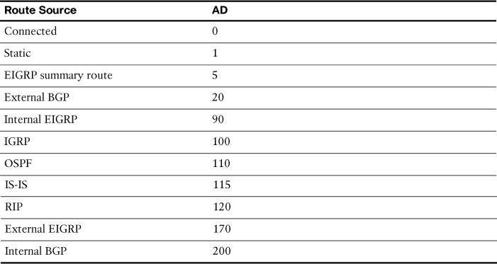
Administrative distance (AD) defines the preference of a routing source. Each routing source—including specific routing protocols, static routes, and even directly connected networks—is prioritized in order of most to least preferable using an AD value. Cisco routers use the AD feature to select the best path when they learn about the same destination network from two or more different routing sources.
The AD value is an integer value from 0 to 255. The lower the value, the more preferred the route source. An administrative distance of 0 is the most preferred. Only a directly connected network has an AD of 0, which cannot be changed. An AD of 255 means that the router will not believe the source of that route and it will not be installed in the routing table.
In the routing table shown in Example 28-1, the AD value is the first value listed in the brackets. You can see that the AD value for RIP routes is 120. You can also verify the AD value with the show ip protocols command, as demonstrated in Example 28-2.
Example 28-2 Verifying the AD Value with the show ip protocols Command
R2# show ip protocols
Routing Protocol is "rip"
Sending updates every 30 seconds, next due in 12 seconds
Invalid after 180 seconds, hold down 180, flushed after 240
Outgoing update filter list for all interfaces is not set
Incoming update filter list for all interfaces is not set
Redistributing: rip
Default version control: send version 1, receive any version
Interface Send Recv Triggered RIP Key-chain
Serial0/0/1 1 2 1
FastEthernet0/0 1 2 1
Automatic network summarization is in effect
Maximum path: 4
Routing for Networks:
192.168.3.0
192.168.4.0
Passive Interface(s):
Routing Information Sources:
Gateway Distance Last Update
192.168.4.1 120
Distance: (default is 120)
Table 28-1 shows a chart of the different administrative distance values for various routing protocols.
IGP Comparison Summary
Table 28-2 compares several features of the currently most popular IGPs: RIPv2, OSPF, and EIGRP.

Routing Loop Prevention
Without preventive measures, distance vector routing protocols could cause severe routing loops in the network. A routing loop is a condition in which a packet is continuously transmitted within a series of routers without ever reaching its intended destination network. A routing loop can occur when two or more routers have inaccurate routing information to a destination network.
A number of mechanisms are available to eliminate routing loops, primarily with distance vector routing protocols. These mechanisms include the following:
![]() Defining a maximum metric to prevent count to infinity: To eventually stop the incrementing of a metric during a routing loop, “infinity” is defined by setting a maximum metric value. For example, RIP defines infinity as 16 hops—an “unreachable” metric. When the routers “count to infinity,” they mark the route as unreachable.
Defining a maximum metric to prevent count to infinity: To eventually stop the incrementing of a metric during a routing loop, “infinity” is defined by setting a maximum metric value. For example, RIP defines infinity as 16 hops—an “unreachable” metric. When the routers “count to infinity,” they mark the route as unreachable.
![]() Hold-down timers: Used to instruct routers to hold any changes that might affect routes for a specified period of time. If a route is identified as down or possibly down, any other information for that route containing the same status, or worse, is ignored for a predetermined amount of time (the hold-down period) so that the network has time to converge.
Hold-down timers: Used to instruct routers to hold any changes that might affect routes for a specified period of time. If a route is identified as down or possibly down, any other information for that route containing the same status, or worse, is ignored for a predetermined amount of time (the hold-down period) so that the network has time to converge.
![]() Split horizon: Used to prevent a routing loop by not allowing advertisements to be sent back through the interface they originated from. The split horizon rule stops a router from incrementing a metric and then sending the route back to its source.
Split horizon: Used to prevent a routing loop by not allowing advertisements to be sent back through the interface they originated from. The split horizon rule stops a router from incrementing a metric and then sending the route back to its source.
![]() Route poisoning or poison reverse: Used to mark the route as unreachable in a routing update that is sent to other routers. Unreachable is interpreted as a metric that is set to the maximum.
Route poisoning or poison reverse: Used to mark the route as unreachable in a routing update that is sent to other routers. Unreachable is interpreted as a metric that is set to the maximum.
![]() Triggered updates: A routing table update that is sent immediately in response to a routing change. Triggered updates do not wait for update timers to expire. The detecting router immediately sends an update message to adjacent routers.
Triggered updates: A routing table update that is sent immediately in response to a routing change. Triggered updates do not wait for update timers to expire. The detecting router immediately sends an update message to adjacent routers.
![]() TTL field in the IP header: The purpose of the Time to Live (TTL) field is to avoid a situation in which an undeliverable packet keeps circulating on the network endlessly. With TTL, the 8-bit field is set with a value by the source device of the packet. The TTL is decreased by 1 by every router on the route to its destination. If the TTL field reaches 0 before the packet arrives at its destination, the packet is discarded and the router sends an ICMP error message back to the source of the IP packet.
TTL field in the IP header: The purpose of the Time to Live (TTL) field is to avoid a situation in which an undeliverable packet keeps circulating on the network endlessly. With TTL, the 8-bit field is set with a value by the source device of the packet. The TTL is decreased by 1 by every router on the route to its destination. If the TTL field reaches 0 before the packet arrives at its destination, the packet is discarded and the router sends an ICMP error message back to the source of the IP packet.
Link-State Routing Protocol Features
Like distance vector protocols that send routing updates to their neighbors, link-state protocols send link-state updates to neighboring routers, which in turn forward that information to their neighbors, and so on. At the end of the process, like distance vector protocols, routers that use link-state protocols add the best routes to their routing tables, based on metrics. However, beyond this level of explanation, these two types of routing protocol algorithms have little in common.
Building the LSDB
Link-state routers flood detailed information about the internetwork to all the other routers so that every router has the same information about the internetwork. Routers use this link-state database (LSDB) to calculate the currently best routes to each subnet.
OSPF, the most popular link-state IP routing protocol, advertises information in routing update messages of various types, with the updates containing information called link-state advertisements (LSA).
Figure 28-1 shows the general idea of the flooding process, with R8 creating and flooding its router LSA. Note that Figure 28-1 shows only a subset of the information in R8’s router LSA.
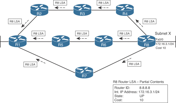
Figure 28-1 shows the rather basic flooding process, with R8 sending the original LSA for itself and the other routers flooding the LSA by forwarding it until every router has a copy.
After the LSA has been flooded, even if the LSAs do not change, link-state protocols do require periodic reflooding of the LSAs by default every 30 minutes. However, if an LSA changes, the router immediately floods the changed LSA. For example, if Router R8’s LAN interface failed, R8 would need to reflood the R8 LSA, stating that the interface is now down.
Calculating the Dijkstra Algorithm
The flooding process alone does not cause a router to learn what routes to add to the IP routing table. Link-state protocols must then find and add routes to the IP routing table using the Dijkstra Shortest Path First (SPF) algorithm.
The SPF algorithm is run on the LSDB to create the SPF tree. The LSDB holds all the information about all the possible routers and links. Each router must view itself as the starting point, and each subnet as the destination, and use the SPF algorithm to build its own SPF tree to pick the best route to each subnet.
Figure 28-2 shows a graphical view of the results of the SPF algorithm run by Router R1 when trying to find the best route to reach subnet 172.16.3.0/24 (based on Figure 28-1).
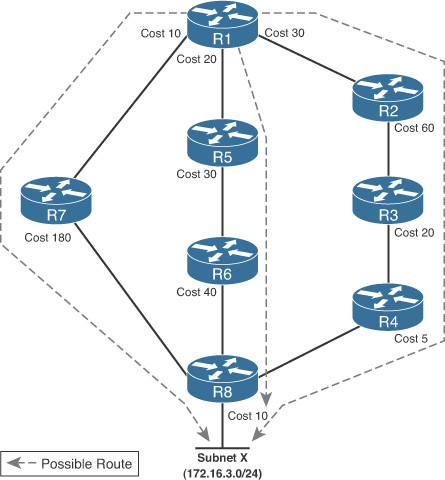
To pick the best route, a router’s SPF algorithm adds the cost associated with each link between itself and the destination subnet, over each possible route. Figure 28-2 shows the costs associated with each route beside the links, with the dashed lines showing the three routes R1 finds between itself and subnet X (172.16.3.0/24).
Table 28-3 lists the three routes shown in Figure 28-2, with their cumulative costs, showing that R1’s best route to 172.16.3.0/24 starts by going through R5.

As a result of the SPF algorithm’s analysis of the LSDB, R1 adds a route to subnet 172.16.3.0/24 to its routing table, with the next-hop router of R5.
Convergence with Link-State Protocols
Remember, when an LSA changes, link-state protocols react swiftly, converging the network and using the currently best routes as quickly as possible. For example, imagine that the link between R5 and R6 fails in the internetwork of Figures 28-1 and 28-2. The following list explains the process R1 uses to switch to a different route:
1. R5 and R6 flood LSAs that state that their interfaces are now in a “down” state.
2. All routers run the SPF algorithm again to see whether any routes have changed.
3. All routers replace routes, as needed, based on the results of SPF. For example, R1 changes its route for subnet X (172.16.3.0/24) to use R2 as the next-hop router.
These steps allow the link-state routing protocol to converge quickly—much more quickly than distance vector routing protocols.
Study Resources
For today’s exam topics, refer to the following resources for more study.
