
12
Digital Signal Processing in Optical Transmission Systems under Self-Homodyne Coherent Reception
Electronic processing is attracting research and development of the enabling technologies for mitigation of impairments at the receiver as equalizer and at transmitters as predistortion. They are thus very important to long-haul transmission systems and networks as well wide-area networks in which the equalizers can be placed at the optical receiver to adaptively equalize any distortion due to different hops in the transmission path in all-optical networks. This chapter introduces the basic concepts of equalization and then gives a case study of equalization of duobinary and minimum shift keying (MSK) modulation formats.
12.1 Introduction
With the advent of digital signal processors and the decrease in the cost of electronic processing systems, electronic signal processing is becoming very attractive for mitigating various impairments that severely affect optical transmission. Equalization and compensation of the impairment effects of the transmission of optical signals through optically amplified systems have been a principal concern for transmission engineering. Compensation of linear and nonlinear dispersion represents a typical and important application of the processing. Over the years, the compensation has been implemented in long-haul transmission with the insertion of dispersion-compensating fibers (DCF) at the end of a transmission span (e.g., standard single-mode fiber [SSMF] or LEA), or a fiber Bragg grating (FBG) with phase fluctuation. These compensating devices would normally suffer appreciable attenuation, and hence an additional optical amplifier must be used to compensate for these lost factors. Thus, additional optical amplifiers are necessary for long-haul transmission systems. Unavoidable accumulated noises of the ASE noise sources from these amplifiers will shorten the transmission distance. Furthermore, the narrow core of a DCF renders it more susceptible to fiber nonlinearity effects. The DCF is also polarization sensitive.
On the contrary, electrical equalization can offer the advantages of more flexibility and lower cost, and a smaller integrated size for the transceiver electronics. Furthermore the programmability of the digital signal processing provides better system management. Thus, if one could compensate or equalize the pulse sequence in the electrical domain either by predistortion or postcompensation, or a combination of both processes, then the elimination of these amplifying processes can be reduced, thus making possible longer transmission reach.
Furthermore, optical networks with different transmission paths carrying lightpaths of different distances due to the different numbers of hops would suffer dispersion and nonlinear effects due to the nature of ultra-high speeds at 10 Gbps or higher. The 10 Gbps Ethernet is coming into the networks in the near future, and there is an urgent demand that inexpensive techniques be available for network implementation. These techniques must be very adaptive and tunable with control signals. Electronic equalization can offer these solutions for high-speed optical networks. Table 12.1 shows the penalty of the eye opening with respect to the bit rate and the length of SSMF when no dispersion compensation is used. This dispersion tolerance becomes very critical when the bit rate is increased. It is important to implement equalization in the electrical domain of digital signal processing, so that it can be tuned or controlled for adaptation to the number of hops of the lightwave channels traveling over the network nodes. These digital signal processing systems for equalization would enhance the received opening eye diagram. Shown in Table 12.1 is the eye opening penalty of some advanced modulation formats due to distortion by chromatic dispersion.
TABLE 12.1
Eye Opening Penalty—Dispersion Tolerance and Equivalent Length of SSM for Different Bit Rates
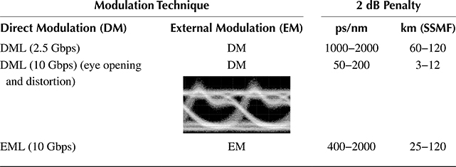
Naturally, the dispersion-limited distance can be improved using optical predistortion techniques such as the control of the chirp of the laser to 200 km SSMF [1] for 10 Gbps, or technique of dispersion-supported transmission to 250 km SSMF [2]. However, these techniques require high complexity of the optical transmitters.
For conventional direct detection receivers, the linear distortion that is induced by chromatic dispersion in the optical domain is transformed into a nonlinear distortion in the electrical signal, which explains why only limited performance improvements can be achieved by using a linear baseband equalizer with only one baseband received signal. This also explains why nonlinear techniques, such as decision feedback equalization (DFE) and maximum-likelihood sequence detection (MLSE), are more effective in combating chromatic dispersion in direct detection receivers. Strictly speaking, the MLSE system attempts neither to compensate the chromatic dispersion effects nor to equalize them, but duly account for these effects in the data detection process.
On the contrary, in a coherent detection system, chromatic dispersion is linear in the electrical signal at the receiver, which is why fractionally spaced equalizers with “complex coefficients” can achieve a performance that is limited only by the number of taps used within the equalizer accounting for the fiber chromatic dispersion only. Recently, with the availability of narrow-linewidth and tunable lasers and ultra-high-speed receivers, coherent lightwave systems have attracted significant attention. However, they have not reached the practical and installation stage so far. This is attributed mainly to the success of wavelength-division multiplexing (WDM) technology with the advent of erbium-doped fiber amplifiers (EDFAs) since the late 1990s. Another reason is the complexity of coherent transmitters and receivers.
The detrimental effect of chromatic dispersion in SSMF can also be reduced by using reduced-bandwidth modulation formats such as optical duobinary signals, single sideband, or vestigial side-band, which can extend the reach of 10 Gbps systems to distances in excess of 200 km, compared with approximately 80 km for conventional NRZ-OOK. In this chapter, optical duobinary signaling is combined with linear electrical pre-equalization schemes [3] to demonstrate the extension of the reach of a 10 Gbps system to several hundred kilometers without any optical chromatic dispersion compensation. In fact, the system reach is influenced by other fiber impairments other than chromatic dispersion. The equalization is based on exploiting the linearity of a coherent lightwave system to move the equalization process to the transmitter, where the data, especially the carrier phase, is still undisturbed. More specifically, the duobinary signal is pre-equalized using two tunable T/2-spaced finite-impulse response (FIR) filters. The outputs of the FIR filters then modulate two optical carriers that are in phase quadrature. Thus, the advantages of coherent receiver equalization are still maintained while utilizing a conventional noncoherent direct detection receiver. Although this chapter focuses on duobinary modulation, this choice is principally driven by the reduced-bandwidth advantage, compared with conventional NRZ-OOK modulation, and the ability to use a conventional direct detection receiver. In principle, electrical pre-equalization can also be applied to other modulation formats for potential improvements.
Duobinary offers the most effective mitigation of the linear dispersion due to its single-sideband property and direct detection at the receiver. Duobinary signaling can also be combined with a proposed electrical pre-equalization scheme to extend the reach of 10 Gbps signals that are transmitted over SSMF. The proposed scheme is based on predistorting the duobinary signal using two T/2-spaced FIR filters. The outputs of the FIR filters then modulate two optical carriers that are then applied to the two parallel MZIM to generate duobinary optical signals. This equalization and duobinary modulation formats for extending the transmission reach are demonstrated in the first section of this chapter with an adaptation of the algorithm given in Ref. [3].
Other equalization systems that would be implemented in the electrical domain include the MLSE equalizers, which have recently received much interest as an effective solution for overcoming the severe distortion caused by the intersymbol interference (ISI) of the optical channels and for improving the signal-to-noise ratio (SNR) performance, thus extending the reach of the optical transmission systems. Most of the studies on the use of nonliner MLSE equalizers have concentrated on amplitude or differential phase modulation formats [4,5 and 6]. However, there are not many reports on the performance of MLSE equalizers for optical transmission systems employing the MSK modulation format.
A narrowband filter receiver with a breakthrough dispersion tolerance limit for the detection of noncoherent 40 Gbps optical MSK transmission system has been proposed and explained in detail in Chapter 8. The performance of this receiver was found to be limited by ISI caused by the differential group delay of the optical channel and the narrow bandwidth of the optical detection filter. In order to combat the ISI, in this chapter, two nonlinear equalizers are proposed and integrated with the narrowband filter receiver for the detection of noncoherent 40 Gbps optical MSK signals. The performances of the proposed schemes are numerically evaluated. The proposed schemes extend the reach of dispersion tolerance of the proposed narrowband optical MSK receiver to ±952 and ±884 ps/nm at BER = 1e−9, or equivalently 52 and 56 km of SSMF with required OSNR of 19 and 23.5 dB, respectively. To the best of the author’s knowledge, these dispersion tolerance limits have not been reached before.
Recently, MLSE equalizer for optical transmission systems employing the MSK modulation format has been reported [4]. The uncompensated distance can equivalently reach up to approximately 960 km SSMF for 10 Gbps transmission. The results are comparable to the distance of 1040 km SSMF as reported in Ref. [5] for IMDD systems. In Ref. [5], up to 8192 trellis states are used. Longer reach for IMDD systems require a very high number of states, which is even infeasible in simulation. Due to large-bandwidth optical filters being used in IMDD systems, noise is not greatly suppressed, leading to high values of required optical-signal-to-noise (OSNR) ratios. In addition, noise distribution in IMDD systems no longer follows a Gaussian profile, which increases the complexity of the equalizer in order to estimate the noise distribution for optimal performance of the Viterbi algorithm. These issues can be effectively mitigated with the introduction of narrowband optical filtering in an optical MSK transmission system.
In this section, we numerically described the possibility of transmission over 1472 km SSMF optical link without in-line dispersion compensation for 10 Gbps optical MSK signals. The achievement is enabled by the integration of 1024-state Viterbi–MLSE equalizer with the noncoherent narrowband frequency discrimination receiver. The proposed receiver mitigates the fiber intersymbol interference (ISI) effectively and greatly reduces the noise floor, thus enabling low OSNR for receiver sensitivity. The simulation results also show significant OSNR improvements with two and four samples per bit over the conventional one sample per bit. Finally, the MLSE equalizer in our proposed scheme can operate optimally due to Gaussian noise distribution [6]. Thus, the complexity of the MLSE equalizer is reduced, compared to the IM/DD systems.
This chapter is organized as follows: the next two sections give a general overview and detailed schemes of equalization whereby the equalizers are placed at the receiver, the transmitter, and a share between transmitters and receiver. Essential expressions of the sampled impulse responses of the equalizer subsystems, the FFE, DFE, and combined nonlinear and linear equalizers are summarized from Ref. [7]. The minimization of the square error in the FFE and DFE is also integrated to optimize the equalization process. The doubling sampling or partial response equalization is also included. Two special cases of equalization—the duobinary and MSK modulation formats—are described in detail in Sections 12.5 through 12.8, using double sampling and MLSE techniques, respectively. Section 12.9 then gives some degree of uncertainty in the equalization process, and the gain in the eye opening penalty, the number of taps, or length of the templates in MLSE schemes are obtained. Finally, the concluding remarks are given.
12.2 Electronic Digital Processing Equalization
Electronic equalization can be implemented with the possibilities of (1) integration of digital signal processing (DSP) at the receive-side; (2) postequalization, placing the equalization DSP at the transmit-side, or predistortion of the optical signals by modification of the electrical signals driving the external modulator; or (3) sharing the equalization function at both the receive-side and transmit-side, that is, using both predistortion and postequalization.
Figure 12.1 shows the generic arrangement of the equalizers at both the transmit-side and receive-side. The equalization processes can occur by using the predistortion at the transmitter (Tx) only or postcompensation at the receive-side (Rx) only, or sharing between the predistortion and postcompensation at both the Tx and Rx sides. Figure 12.2 shows the equalization processing both in the optical and electronic domains at the receiver and transmitter sides. The optical equalization works with the field of the lightwaves, while the electronic processor works with the electrical signals obtained from the conversion of the optical intensity of the signals, except for the case of coherent reception, the received signals are directly related to the phase in the electrical at the driving input of the optical modulator. A typical layered optical network using IP over WDM is shown in Figure 12.3, in which the equalizer is used to equalize any distortion residual from the optical compensator—for example, phase ripple of the phase group delay of the FBG dispersion compensator, or different traveling hops of the lightpaths. It has been noted that electronic equalizers do not suffer the problems of over-dispersion as in the case of optical compensators, as the electrical type deals with the intensity while the optical type deals with the field and over-compensation or under-compensation, due to the variation of the residual dispersion in different lengths of hops of the lightpaths. Figure 12.4 [4] also shows a typical light of a wavelength channel traveling through the network. The insert in this figure extends the dispersion tolerance with and without equalization. Optical equalizers can be shared by the channels of different wavelengths, while an electronic equalizer is normally integrated into a receiver for a specific channel.
When the equalizer is operating at the receiver, then this postequalization would take the advantage of the knowledge of all distortion effects and deals with the signals depending on the intensity. The distorted signals can then be equalized. If any unexpected distortion occurs, this postequalization can be adaptive to equalize the pulse sequence. On the contrary, an equalizer placed at the transmit-side is processing the lightwave by creating a predistortion on the phase of the carrier. Note that the channel is purely phase distortion, and thus the sequence can be electrically predistorted before driving the external modulator to chirp the phase in such a way that opposes the chirping by the group velocity of the optical fiber.

FIGURE 12.1 Arrangement of electronic DSP for equalization in optical transmission systems. Electronic DSP for predistortion, electronic DSP at the Rx is for postequalization and shared predistortion and postequalization at the Tx and Rx: (a) equalization at the transmit-side, (b) equalization at the receive-side, and (c) equalization shared between the Tx and Rx sides.
The postequalization processing usually requires a number of samples to ensure sufficient data for its equalization technique. The higher the number of samples, the better the equalized sequence. However, for long-haul optical transmission systems, the pulse may be very dispersive and the samples may suffer significant distortion. In order to assist the postequalizer, a predistortion compensator may be placed at the transmitter to share the equalization functionality with the postequalizer to extend the reach of the optical transmission system.

FIGURE 12.2 Typical structure and position of the DSP equalizer of a receive-side equalized optical system. Both optical and electronic equalization processors are integrated. O_EQ = optical equalizer; T_DC-tunable dispersion compensator; PMDC = polarization-mode dispersion compensation; O/E = optical to electrical converter; DFE = decision feedback equalizer; FFE = feed-forward equalizer; MLSE = maximum-likelihood sequence estimator.

FIGURE 12.3 Typical layered graph model for IP over WDM network with optical receivers and equalizers.

FIGURE 12.4 Typical lightpaths of optical networks and dispersion tolerance without and with electrical equalization. (From N. Alic et al., Opt. Express, Vol. 13, No. 12, pp. 4568–4579, 2005.)
TABLE 12.2
Dispersion Tolerance and Equivalent Length of SSM for Different Modulation Formats and Equalization Techniques and Improved Factors

The benefit of equalization does also depend on the modulation format, as the algorithm must be adapted to the mode of modulation, for example, amplitude, phase, or frequency shift keying. Table 12.2 shows the improvement factors of the equalization techniques on different modulation formats using amplitude shift keying. The duobinary is a tri-level modulation format using both amplitude and phase to represent the levels. However, its detection is intensity based and thus included here.
12.3 System Representation of Equalized Transfer Function
12.3.1 Generic Equalization Formulation
12.3.1.1 Signal Representation and Channel Pure Phase Distortion
Given that the SMF is a pure phase distortion, the equalization deals with the processing of sampled amplitude or phase of the recovered signals pending on the modulation formats whether its amplitude, phase, or frequency is altered. This section gives a brief strategy of development of the requirement on the transfer function of the equalized system and associate filters. It is essential that the impulse response of the channel (the single-mode optical fiber) be obtained in order to specify the equalization subsystems. Thus, this section gives an analytical derivation of the pure distortion channel. Both the impulse and step responses of the fiber channel are analytically derived.
Let the impulse response of the channel (the single-mode optical fiber) be y(t); then the z-transform of the impulse response with a sampling time equal to the bit period is given by
y(nT)=[y0y1....yg00....0]Y(z)=y0+y1z−1....+ygz−g(12.1)
with n ≥ 2g + 1 and yi are complex valued.
Under a purely phase distortion, the channel lost no energy, and hence the conservation of energy requires that
n∑i=0|yj|2=1(12.2)
with the total energy contained in the impulse assumed to be unity.
Now consider the input signals having complex-valued sampled components, such as the QAM optical signals that comprise two DPSKs in phase quadrature or two AM signals in quadrature, one of which carries the data symbols {s1,i}. Each AM signal is associated with the corresponding modulator and demodulator, to recover back to the baseband channel. For advanced modulation formats, the detection can be incoherent or coherent. Under coherent detection, the impulse response takes the amplitude and preserves its phase, while for incoherent or direct detection, the impulse response is the result of the beating of different components of the response in the photodetection process, and its response follows intensity-based square law detection. In this case, the response can be estimated by considering the Gaussian distribution with the pulse-spreading factor.
The input signals can now be written as
si=s0,i+js1,i(12.3)
with j = (−1)1/2, both s0,i and s1,i can independently take on any one of the different m values
-(m-1)k, -(m-3)k,... , (m-1)k(12.4)
An element of the QAM signal carrying the data symbol si is itself the sum of two double-sideband-suppressed carrier AM signal elements in phase quadrature, carrying the data symbols s0,i and s1,i.
The output signals can be real or complex valued. The sequence of the signals at the output of the channel is, of course, given by the sequence of samples at the output of the samplers. The real and imaginary parts of this sequence are samples of the respective baseband signals at the outputs of the two constituent parallel channels that make up the linear baseband channel. It can now be seen that if the sampled impulse response of the linear baseband channel is real, then there is no coupling between the two parallel channels; the distortion of these two channels are the same and can be determined as for ASK signals. On the contrary, if they are complex valued, the coupling is introduced between the two constituent channels by the imaginary parts of the components of the sampled impulse response. The impulse response of a single-mode optical fiber is purely complex-valued and will be described in the following section.
When the channel introduces pure phase distortion, it introduces a unitary transformation into the transmitted signals [8], such that the received signal elements corresponding to the resultant (complex valued) transmitted signal elements are orthogonal. An orthogonal transformation is a special case of unitary transformation where all signals are real valued.
Under coherent detection, the detected signals are given by
ri=siy0+wi(12.5)
where we have assumed, without loss of generality, that the impulse response takes only a non-zero value y0, and wi is the noise contributed to the signal. The noise is statistically independent Gaussian random variables with zero mean and variance σ2. Thus, we have
ri=s0,iy0+js1,iy0+wi(12.6)
Obviously, the received signals must be detected with both the real and imaginary parts. Thus, in the absence of noise, we have
|ri|2=s20,i+s21,i(12.7)
Since the impulse response is of pure phase distortion, then the absolute value of components of the sampled time response is unity, and thus when the input signals are convolved with the impulse response, the phase of the components of the received signals are rotated by a fixed amount of phase.
This is equivalent to the reverse of the components of the impulse response pivoting around the central value at t = 0 by the complex conjugates; thus, the impulse sequence can be written as
yi=yi*y(nT)=[y0y1....0......y*my*m−1....y*1](12.8)
Alternatively, we can state that whenever there is a reversal of the complex-conjugate of a sequence pivoted around its components at t = 0, then the sequence represents a pure phase distortion. Thus, when convolving the sequence with its original one gives a sequence all of whose components are zero except for the component at time t = 0 which is unity.
12.3.1.2 Equalizers at Receiver
12.3.1.2.1 Zero-Forcing Equalization
The equalizer shown in Figure 12.5 is a DFE, which is a nonlinear equalizer in contrast to the linear filter. A linear filter usually consists of a transversal feed-forward equalizer (FFE) that delays the signal by time interval T in which the delayed signals are tapped and multiplied with desired coefficients and then added to form an equalized output. The nonlinear DFE discussed in this chapter is structured with both linear FFE and nonlinear DFE. A zero-forcing equalizer operates as follows.
The linear FFE partially equalizes the signal by setting to zero all components of the channel-sampled impulse response preceding that of the largest magnitude, without changing the relative values of the remaining components. The nonlinear equalizer then completes the equalization process to give accurate equalization of the channel. The equalizer is nonlinear because the detector (or slicer) is a nonlinear device.
Now, let yl be the largest-magnitude component of the impulse response (Equation 12.1); then, the z-transform of the linear FFE of (m+1)-taps is given by
C(z)=c0+c1z-1 ....+cmz−m(12.9)

FIGURE 12.5 Schematic of a nonlinear feedback equalizer following an optical receiver with (a) feed-forward transversal filters at the input and at the feedback path (FFE-DFE), (b) linear feed-forward transversal filter (FFE), and (c) combining FFE and DFE and a slicer for equalization.
Such that
Y(z)C(z)≈z-h(12.10)
where h is a nonnegative integer in the range (m + g). It is also assumed that the frequency transfer response Y(z) does not have zeros on the unit circle of the z-plane.
Now, let the transfer function of the (n + 1) tap FFE filter D in Figure 12.5 be
d(nT)=[d0d1....dn]D(z)=d0+d1z−1....+dnz−n(12.11)
The required sampled impulse response of the combined system consisting of a cascade of the channel and the linear filter D is given by the (g−l + 1)-component row vector
E=[ 1 yl+1yl yl+2yl yl+3yl ygyl ]E(z)=1+yl+1ylz-1+yl+2ylz-2+yl+3ylz-3 ...+ ygylz-g+1...(12.12)
Clearly, E is obtained by removing the first l components and dividing each of the components by yl. As yl is the maximum magnitude, we have all the coefficients of the filter E less than unity. D(z) can now be written as
D(z) = E(z)C(z)
then
Y(z)D(z)=Y(z)C(z)E(z)=z-hE(z)(12.13)
The z-transform of the (i+1)th transmitted signal element is siz−i, and thus the z-transform of the (i + 1)th received signal element at the output of the linear filter D is given by
siz-i-hE(z)=siz-i-h(1+yl+1ylz-1+yl+2ylz-2+yl+3ylz-3...+ygylz-g+1)(12.14)
It is thus observed that, whenever there is a nonzero term, there would be intersymbol ISI between the signal elements at the output of the linear filter. This ISI is then removed in the nonlinear equalizer that equalizes the z-transform z−hE(z), as given earlier. Clearly, the nonlinear DFE follows that of Figure 12.2 with the linear FFE with the number of taps of (g−l), with the tap gain coefficients of (instead of the tap coefficients indicated in Figure 12.2b).
yl+1yl,yl+2yl,yl+3yl,...ygyl(12.15)
At the instant (i + h)T, the input to the substractor is given as
vi+h=si+yl+1ylsi-1+yl+2ylsi-2+yl+3ylsi-3+... +ygylsi-g+l+ui+h(12.16)
where s′i−j
xi+h≃si+ui+h(12.17)
when xi+h > 0, s′i=k
ui+h=n∑j=0wi+h-jdj(12.18)
The noise components are statistically independent Gaussian variables with zero mean and a variance, and thus we have the total variance of the noise component of the detected signal as
η=σ2n∑j=0d2j=σ2|D|2(12.19)
where |D| is the Euclidean length of the vector D. Thus, the probability of error of the detection of si, given the correct detection of si−1, si−2,…, si−g+l, can be approximately given as
Pe=∞∫k1√2πη2e-u22η2du=Q(kη)=Q(kσ|D|)(12.20)
where k is the average total amplitude of the signal at the output of the receiver. The equalizer presented in this section can be optimized to reduce the probability of error further—for example, the use of two cascaded transfer functions to replace the equivalent transfer function of the fiber, where the linear equalizer takes on one part and the other by the nonlinear equalizer. One could thus reduce the number of taps of the linear FFE. The lesser the number of taps, the better the demands puts on the electronic processor operating very high speeds.
12.3.1.2.2 Equalization that Minimizes Mean Square Error (MSE Equalizer)
Both FFE and DFE can equalize and minimize the error contributed by the noise and distortion that would generally offer a more effective degree of equalization than an equalizer that minimizes peak distortion. Such an equalizer minimizes the main difference between the actual and ideal sampled values at its output for a given of taps for the case of FFE. For DFE, the minimization of the error occurs at the point where the feedback linear FFE and that at the output of the linear filter as shown in Figure 12.5.
Under linear equalization, we recall that the channel-sampled transfer function given in Equation 12.1 of the sampled impulse response of the channel and the equalizer is given by the (m + g + 1)th row vector
E=[e0e1 .... .... .... em+g](12.21)
The ideal value of the sampled impulse response of the channel and the equalizer is given by (m + g + 1)-component row vector

where h is an integer and is within the range (m + g). The minimization is thus conducted so that the expected mean value
E[(xi+h-si)2]=k2|E-Eh|2+σ2|C|2(12.23)
where k2 E − Eh|2 and σ2|C|2 are the mean square error (MSE) terms in the received signals xi+h due to ISI and due to the Gaussian noise, respectively, and C is the sampled impulse response of (m + 1)-component row of the FFE, denoted by
C=[c0c1 .... .... .... cm](12.24)
Under nonlinear DFE, the minimization occurs at the error substractor as shown in Figure 12.5; that is, there needs to minimize the MSE of the equalized signals as the expected value of the mean square value which can be expressed as
ε=E[(xi+h-si)2](12.25)
The data symbols si−1, si−2,…,si−μ can be correctly detected by adjusting the coefficients of the FFE filters and then those of the FFE of the feedback DFE. The sampled impulse responses of these filters can be expressed as
D=[d0d1 .... .... .... dn](12.26)
E=[e0e1 .... .... .... en+g](12.27)
F=[f0f1 .... .... .... fμ](12.28)
S=[sisi−1si−2 .... .... .... si−n−g](12.29)
where E is the sampled impulse of the fiber channel and the linear equalizer FFE D, and S is the sampled signal correctly detected at the output of the equalizer. The signals at the input of the detector in Figure 12.5 at time t = (i + h)T are given by

The MSE can thus be written as [9]
ε = k2|B|2 + σ2|D|2
with

The data symbols are assumed to be statistically orthogonal with zero mean and variance k2. The DFE feedback nonlinear equalizer is assumed to have μ taps in the filter F. This is the lowest number of taps whereby exact decision-directed cancellation can be achieved of all ISI components in xi+h., involving data symbols si−1, si−2,...,si−μ that have been detected.
After a number of manipulation steps, the MSE can be obtained as
ε=k2[1-EhZT(ZZT+o2k2I)-1ZETh](12.32)
where Z = [(n + 1) × (n + g + 1)], derived from [Yc] = convolution matrix of the sampled impulse response. The matrix Z can be written as
Z=[y0y1y2...........0....0....00y0y1..........0....0....000y2............0....0....0...........................0....0....0000......y0y1y20...00000y0y1y2...000000y0y1...0000000y0.....0](12.33)
12.3.1.2.3 Nonlinear Equalization that Minimizes SNR
An optimum DFE can be considered as a DFE that further minimizes the BER in the detected signals for a given DFE structure. As previously assumed, the z-transform of the fiber channel in intensity has no zeros or roots on the unit circle of the z-plane. Thus, we have the sampled impulse response of the channel, and the FFE of the DFE is given by
Y(z)C(z)≃z-horC(z)≃z-hY-1(z)(12.34)
Then the FFE D of the DFE can be composed of the FFE C and a filter E under the constraint that
Y(z)D(z)≃z-hE(z)(12.35)
where E(z) = [e0, e1, ... , en−m]. The nonlinear equalizer of Figure 12.5 equalizes E(z) so that the linear FFE of the feedback path F has (n − m) taps with the gains equal, respectively, to the components ei, e2, ... ,en–m of the vector E.
The signals at the output of the linear filter D, at the instant t, is thus given by (i + h)T
vi+h≃si+si-1e1+si-2e2+......+si-n+men-m(12.36)
With the corrected detection of the input signals si–t, the equalized signals at the output of the DFE can be written as
xi+h≃si+ui+h(12.37)
So,whenxi+h={>0....s′i=k<0.....s′i=−k
the noise component ui+h is a Gaussian random variable as assumed previously with zero mean and variance of η, given as
η=σ2|D|2(12.38)
Thus, the BER can be obtained as
Pe=∞∫k1√2πη2e-u22η2du=Q(kη)=Q(kσ|D|)(12.39)
So, it is necessary to minimize the Euclidean length of the linear FFE filter or find the minimum number of taps of the filter that still allow the maximizing of the SNR. Thus, the DFE should be adjusted to minimize the vector length |D|. This minimization can be implemented as follows. This minimization can be done at the linear filter D of the DFE such that
|D|=|G0-LM|(12.40)
With
G0=[0c0c1c2........cm0..........0]M=[0c0c1c2........000c0.........00................................cm........00cm−1........00cm−2 cm−1cm]L=[−e1−e2...........−en−2−m−en−1−m−en−m](12.41)
The task is now adjusting L so that minimization of the vector length D happens.
12.3.1.2.4 Case Study of Equalization Schemes
This section gives a case study of direct detection with the impulse response of the SMF or the residual dispersion of a dispersion-managed transmission system. The sampled impulse response is a real impulse response after the photodetector and electronic preamplifier. This impulse response follows a Gaussian distribution with the broadening of the impulse at the e−1 value of the maximum peak by an amount given by
Δτ=D⋅L⋅B3dB(12.42)
where B3dB is taken as the 3 dB bandwidth of the power spectra of the signals under different modulation formats.
A typical dispersive impulse at the instant t = iT can be given by
ri=0.3si+si-1=wi(12.43)
where the data symbol {si} is statistically independent and equally likely to have either value ±k and {wi} are statistically independent Gaussian random variable with zero mean and a variance σ2. Effectively, the impulse response of the fiber transmission disperses to 30% of the peak amplitude at the output of the electronic preamplifier. We can compare the tolerance to noises of the following equalization processes: (a) a simple threshold level detector, (b) a linear FFE, (c) a purely NL DFE, (d) linear and nonlinear equalization of two factors of the channel, and (e) optimum DFE.
12.3.1.2.4.1 Nonequalization Direct Detection
At a high SNR, practically all the errors occur when si+1 = −si, that is, when ri+1 = 0.7si + wi. Thus, the BER can be derived as
Pe=∞∫0.7k1√2πσ2e-u22σ2du=Q(0.7kσ)(12.44)
(a) Linear Equalization
The sampled impulse response of the fiber channel is given by the two component sequence Y = [0.3, 1], so that the z-transform of the sequence is given by Y(z) = 0.3 + z−1. Now, assuming that a six-tap linear FFE is designed for the equalization so as to minimize the peak distortion is M(z) = 1 + 0.3 z−1, then the equalizer with a six-tap FFE can be found by taking a long division of (1 + 0.3 z−1)−1. The long division gives
N(z)=1-0.3z-1+0.09z-2−0.027z−3+0.0081z-4-0.00243z-5(12.45)
Thus, the C(z) of the FFE can be obtained by reversing the order of the N(z) as
C(z)=1.z-5-0.3z-4+0.09z-3-0.027z-2+0.0081z-1-0.00243(12.46)
Hence, the z-transform of the cascaded channel and the FFE is simply given as
C(z)Y(z)=0.000729+z-6≃z-6(12.47)
Thus, the equalized pulse at the instant t = (i + 6)T is
xi+6=1wi+1-0.3wi+2+0.09wi+3-0.027wi+4-0.0081wi+5-0.00243wi+6(12.48)
The Gaussian noise can be estimated as
η=1wi+1-0.3wi+2+0.09wi+3-0.027wi+4+0.0081wi+5-0.00243wi+6(12.49)
Thus, the noise variance is obtained as
η2=σ2(1-0.3+0.09-0.027+0.0081-0.00243)=1.0989σ2(12.50)
Thus, the probability of error is given by
Pe=∞∫k1√2πη2e-u22η2du=Q(kη)=Q(k1.0989σ)=Q(0.9539kσ)(12.51)
(b) NL DFE
On receiving the signals ri, the NL DFE determines s′i−1
xi=0.3si+wi(12.52)
and si is now detected from xi as follows
xi+h={>0si′=k<0si′=-k (12.53)
An error occurs here in the detection of si when wi has a magnitude greater than 0.3 k and the opposite sign to si. Thus, the probability of error of the equalized signals is given by
Pe=∞∫k1√2πη2e-u22η2du=Q(kη)=Q(0.3kσ)(12.54)
(c) Linear and Nonlinear Equalization
The linear and nonlinear equalization of the two factors here would degenerate into a linear equalizer since the impulse response z-transform of Y(z) does not have zero in the outside region of the unit circle in the z-plane. Thus, the probability of error is the same as in the case (b), that is
Pe=Q(0.9539kσ)(12.55)
(d) Optimum DFE
The first FFE of the nonlinear equalizer performs an orthogonal transformation on the receive signals, such that the z-transform of the channel and the filter becomes
Y(z)D(z)≃z-h(1+0.3z-1)(12.56)
The filter does not change the SNR and the noise property or any distortion of the amplitude of the received signal. Its output signal at t = (i + h)T is
vi+h=si+0.3si-1+ui+h(12.57)
where ui is a Gaussian random variable of zero mean and a variance of σ2. Thus, the probability of error is
Pe=∞∫k1√2πσ2e-u22σ2du(12.58)
On receiving vi+h, the nonlinear filter has formed 0.3s′i−1
xi+h=vi+h-0.3s′i−1(12.59)
Then fed to the detector or decision device, the correct detected signal and the equalized signal becomes
xi+h=sj+ui+hwhenxi+h={>0...s′l=k<0.....s′i=−k(12.60)
An error occurs in the detection of si from xi+h when ui+h has a magnitude greater than k and opposite in sign to si so that, regardless of the sign of si, the probability of detection of si can be approximately given as
Pe=∞∫k1√2πσ2e-u22σ2du=Q(kσ)(12.61)
Thus, from the preceding analytical estimation of the probability of error as a function of the SNR k/σ, we can see that the resilience to noise of the optimum DFE is best with about 0.4 dB.
The pure nonoptimized nonlinear DFE can suffer −2.7 dB under direct detection without equalization and 0 dB for linear FFE.
12.3.1.2.5 Nonlinear Equalization under Severe Amplitude Distortion
The maximum-likelihood sequence estimation (MLSE) is considered as the detection of the transmitted sequence with minimum probability of error, and it depends on the coding and modulation formats of the signals. This method is further explained in detail in Section 12.7.
12.3.1.3 Equalizers at the Transmitter
Consider an arrangement where the equalizer acts as a predistortion and is placed at the transmitter. The nonlinear equalizer in this case converts the sequence of data symbols {si} into a nonlinear channel {fi} at the output of the transmitter, normally an optical modulator driven by the output of the nonlinear electrical equalizer as shown in Figure 12.1b and remodeled as shown in Figure 12.6.
These symbols are sampled and transmitted as sampled impulses {fi δ(t−iT)}. The SNR in this case is given by E[f2i]/σ2
F(z)=M[S(z)-F(z)(y-10Y(z)-1](12.62)
where S(z) is the z-transform of the sampled input signals, and Y(z) is the z-transform of the channel transfer function. Then, the z-transform at the output of the nonlinear processor at the receiver can be written as
X(z)=M[F(z)Y(z)+W(z)]=M[F(z)(y-10Y(z)-y-10W(z)]or X(z)=M[S(z)-y-10W(z)](12.63)
That is, xi=M[y-10ri]=M[si+y-10wi]
The nonlinear processor M operates as a modulo-m as
M[q]=[(q+2k) modulo−4k]-2k=q-4jk-2k≤M[q]≤2k(12.64)

FIGURE 12.6 Schematic of a nonlinear feedback equalizer at the transmitter.
Thus, an error would happen when
(4j-3)k≤y-10wi≤(4j-1)k ∀j(12.65)
The probability of error is then given as
Pe=2∞∫k1√2πy-20σ2e-w22y20σ2dw=2Q(k|y0|σ)(12.66)
12.3.1.4 Equalization Shared between Receiver and Transmitter
Long-haul transmission requires equalization so that the extension of the transmission can be as far as possible. Equalization at the receiver can be supplemented with that at the transmitter to further increase the reach.
The equalizer at the transmitter of the preceding section can be optimized by inserting another filter at the receiver. Consider the channel transfer function Y(z) that can be written as a cascade of two linear transfer functions Y1(z) and Y2(z) as
Y(z)=Y1(z)Y2(z)with {Y1(z)=1+p1z−1+........+pg−fz−g+fY2(z)=q0+q1z−1+........+qfz−f(12.67)
Y1(z) has all the zeros inside the unit circle and Y2(z) all outside the unit circle. Then we could find a third system with a transfer function that has all the coefficients in reverse of those of Y2(z), given as
Y3(z)=qf+qf-1z-1+......+q0z-f(12.68)
with the reverse coefficients, the zeros of the Y3(z), now lying inside the unit circle.
The linear FFE filter D of the nonlinear filter formed by cascading an FFE and a DFE as shown in the preceding text can minimize the length of the vector of D and minimizing e0 can be implemented, provided that
D(z)=z-hY-12(z)Y3(z)(12.69)
which represents an orthogonal transformation without attenuation or gain. The linear equalizer with a z-transform Y2(z)Y3−1(z) is an all-pass pure phase distortion.
This transfer function of the all-pass pure phase distortion is indeed a cascade of optical interferometers, known as half-band filters [10]. This function can also be implemented in the electronic domain. The equalizer can then be followed by an electronic DFE. Hence, the feedback linear filter F(z) in Figure 12.5 can be written as
F(z)=Y1(z)F3(z)(12.70)
The probability of error can be similarly evaluated and given by
Pe=∞∫k1√2πy-20σ2e-w22y20σ2dw=Q(k|qf|σ)(12.71)
where qf is the first coefficient of Y3(z).
12.3.1.5 Performance of FFE and DFE
The performance of a linear equalizer using an FIR filter with a different order is shown in Figure 12.7 with the penalty of eye opening versus the dispersion factor [11]. The higher the order of the FIR, the better the equalization of the distorted impulse, or the longer the length of the SSMF that the signals can propagate. While the receiver without equalization would suffer an EOP of at last 12 dB, a seventh-order FIR filter can equalize the distorted signals over 150 km with only 1 dB EOP.
Figure 12.8 shows the EOP versus the fiber length (SSMF) for the case of nonlinear equalizer with an FFE and a DFE with the orders of second and third, respectively. With 1 dB EOP, the FFE and DFE combined nonlinear filter can extend the transmission of 10 Gbps NRZ-ASK to 150 km, and to 300 km with nonlinear correction.
Figure 12.8 shows the EOP of modulation formats of NRZ-ASK and NRZ duobinary using FIR of number of taps of 3 and 16 with the distortion of signals. Up to 400 km, SSMF transmission is possible with the equalized system for 1 dB EOP.
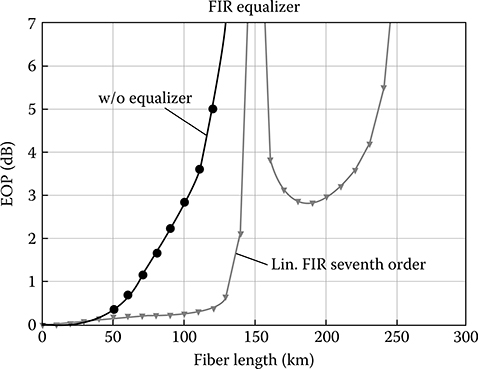
FIGURE 12.7 Eye opening penalty as a function of the dispersion tolerance in kilometers of SSMF without and with linear equalizer FIR.

FIGURE 12.8 Eye opening penalty as a function of the dispersion tolerance in kilometers of SSMF without and with linear and nonlinear equalizer FFE-DFE.
In the next section, the impulse response of the fiber is described; especially, it is proven that it is a purely imaginary response as the channel is a pure phase distortion. The impulse response for intensity distortion can be found very easily with Gaussian shape approximation (see Chapter 2) and the broadening of the impulse can be estimated from Equation 12.42.
It is then followed by a detailed description of the equalization using MLSE for continuous phase FSK or optical MSK modulation schemes.
12.3.2 Impulse and Step Responses of the Single-Mode Optical Fiber
The treatment of lightwaves through SMF has been well documented, as given in Chapter 4. In the following, we shall restrict our study to the linear region of the media. Furthermore, the delay term in the transmittance function for the fiber is ignored, as it has no bearing on the size and shape of the pulses. We can thus model the fiber simply as a quadratic phase function. The input–output relationship of the pulse can therefore be depicted as in Figure 12.9.
Equation 12.1 expresses the time-domain impulse response h(t) and the frequency-domain transfer function H(ω) as a Fourier transform pair
h(t)=√1j4πβ2exp(jt24β2)↔H(ω)=exp(-jβ2ω2)(12.72)
where β2 is known as the group velocity dispersion (GVD) parameter. The input function f(t) is typically a rectangular pulse sequence; the parameter β2 is proportional to the length of the fiber. The output function g(t) is the dispersed waveform of the pulse sequence. The electro system of Figure 12.9 is an exact analogy of diffraction in optical systems (see Ref. [12], item 1, Table 1 of Chapter 2, p. 14). Thus, the quadratic phase function also describes the diffraction mechanism in one-dimensional optical systems, where the distance x is analogous to time t. The establishment of this analogy affords us to borrow many of the imageries and analytical results that have been developed in the diffraction theory. Thus, we may express the step response s(t) of the system H(ω) in terms of Fresnel cosine integral C(t) and Fresnel sine integral S(t) as follows
s(t)=∫t0√1j4πβ2exp(jt24β2)dt=√1j4πβ2[C(√1/4β2t)+jS(√1/4β2t)](12.73)

FIGURE 12.9 Representation of the quadratic phase transmittance function in frequency and time domain.
withC(t)=∫t0cos(π2τ2)dτS(t)=∫t0sin(π2τ2)dτ(12.74)
Using the electro-optical analogies, one may argue that it is always possible to restore the original pattern f(x) by refocusing the blurry image g(x) (e.g., image formation, item 5, Table 2-1, [12]). In the electrical analogy, it implies that it is possible to compensate the quadratic phase media perfectly. This is not surprising. The quadratic phase function H(ω) in Figure 12.1 is an all-pass function, it is always possible to find an inverse function to recover f(t) from g(t). Express this differently in information theory terminology: the quadratic phase channel has a theoretical bandwidth of infinity; its information capacity is infinite. Shannon’s channel capacity theorem states that there is no limit on the reliable rate of transmission through the quadratic phase channel.
The picture changes completely if the detector/decoder is allowed only a finite time window to decode each symbol—for example, detection using frequency discrimination techniques for continuous phase frequency shift keying (CPFSK), in which a narrow optical filter is used to extract the carrier frequency representing the bits “1” or “0.” In the convolutional coding scheme, for example, it is the decoder’s constraint length that manifests as the finite time window. In adaptive equalization schemes, it is the number of equalizer’s delay elements that determines the decoder window length. Since the transmitted symbols have already been broadened by the quadratic phase channel, if they are next gated by a finite time window, the information received could be severely reduced. The longer the fiber, the more the pulses are broadened, and the more uncertain it becomes in the decoding. It is the interaction of the pulse broadening on one hand, and the restrictive detection time window on the other, that gives rise to the finite channel capacity.
Figure 12.10a shows the impulse response of Gaussian pulse transmission of 100 Gbps pulse sequence through an SMF of length L = 200 km, dispersion = 0e−6 s/m2; (a) dispersion slope S = +0.06e + 5 s/m3, while Figure 12.10b shows its response over L = 2 km of the same dispersion factor and dispersion slope. It is noted from Equation 12.72 that the impulse response is a pure phase function, and thus phase distortion. The oscillation of the tail of the impulse response for long fiber indicates the phase chirping of the lightwave carrier in the advanced region of time-dependent pulses. Over a short length of fiber the Gaussian pulse remains with minimum change of the phase underneath its envelope. Figure 12.10c shows the impulse tail oscillation on the other side when it propagates through a dispersion-compensated 200 km fiber span with a total residual dispersion of −8.5 ps/nm that is typically found optically amplified fiber transmission system.
The step response (Equation 12.73) consists of the in-phase and quadrature-phase components. Figure 12.11a through c shows the pulse and step responses, its frequency spectrum, and step response after propagating through 1 km SSMF. The overshooting of the lightwave carrier modulated pulse occurs mostly near its edge that indicates that for the detection of the frequency shift keying modulation (FSK) format would be significantly influenced if the frequency filtering is implemented at the pulse center to obtain the best BER and the receiver sensitivity of the optical systems.
12.4 Electrical Linear Double-Sampling Equalizers for Duobinary Modulation Formats for Optical Transmission
In general, chromatic dispersion is a time-varying impairment mainly because of temperature variations. Implications can be quite critical for 40 Gbps systems that have tight chromatic dispersion tolerances. For 10 Gbps systems, the chromatic dispersion tolerance is far less stringent than 40 Gbps systems (approximately 1000 ps/nm for a 1 dB power penalty). A variation of approximately 0.15 ps/nm/km over the temperature range from 40°C to 60°C. Compared with a typical value for of 17 ps/nm/km, the variation can be neglected. Therefore, it can be assumed, for our immediate purposes, that chromatic dispersion is a static impairment that can be accurately modeled, and hence static equalizers can be utilized. The ideal zero-forcing equalizer is simply the inverse of the channel transfer function given in Chapter 3. Thus, the required equalizer transfer function for the equalizer Heq(f) is given by

FIGURE 12.10 Gaussian pulse transmission of 100 Gbps pulse sequence through an SMF of length L = 2 km, dispersion = 0e−6 s/m2: (a) dispersion slope S = +0.06e + 5 s/m3; fiber length = 200 km; (b) L = 2 km dispersion = 17e−6 s/m2 and S = +0.06e + 5 s/m3; (c) over 200 km SSMF and completely compensated with a mismatch of −8.5 ps/nm dispersion; and (d) enlarged responses with a dispersion slope of DCF = 0.3e + 5 s/m3. Note the oscillation of the tail of the impulse response.
withHeq(f)=H−1f(f)=e+jαf2α=πDLλc2(12.75)
However, this transfer function does not maintain conjugate symmetry, that is
Heq(f)≠H-1eq(-f)(12.76)

FIGURE 12.11 Rectangular pulse transmission through an SMF, near-field response: (a) pulse response; (b) spectrum of pulse in (a); (c) step response, note horizontal axis—unit normalized with time unit; and (d) enlargement of chirping of pulse at the edge due to dispersion slope.
Thus, the impulse response of the equalizing filter is complex, as shown in the previous section (Equation 12.2). Consequently, this filter cannot be realized by a baseband equalizer using only one baseband received signal, which explains the limited capability of linear equalizers that are used in direct detection receivers to mitigate chromatic dispersion.
On the contrary, it also explains why fractionally spaced linear equalizers, especially the double-sampling type that are used within a coherent receiver, can potentially extend the system reach to distances that are only limited by the number of equalizer taps. However, the nonideal effects such as the laser phase noise and the fiber nonlinearity, which eventually set a limit on the maximum achievable transmission distance, should also be taken into account. The equalizer in a coherent receiver, most of the complexity can be avoided at the receiver by an equalization process at the transmitter. The required filter would thus have complex coefficients, and thus the predistorted data have to modulate two optical carriers that are in phase quadrature.
Although the concept of using two optical carriers that are in phase quadrature is not a conventional one, its practical feasibility was shown in Chapter 4, where two orthogonal optical carriers were used to obtain an optical differential quadrature phase shift keying (ODQPSK) transmission system. To determine the required equalizer coefficients, the simulation setup in Figure 12.12 [4] can be used, where an adaptive algorithm is used to adaptively adjust the FIR filter coefficients to their optimum values. The adaptive algorithm adjusts the FIR filter taps to compensate not only for chromatic dispersion but also other linear dispersion effects such as PMD and any other phase–delay-type filter such as phase ripples of chirp FBGs. Once the filter taps converge to their optimal values, the linearity of the system allows transferring the filter to the transmitter side, where it acts as a predistortion filter. The proposed predistortion scheme is depicted in Figure 12.12. The optical transmitter for duobinary is formed using two parallel MZMs and a π/2 optical phase shift, as shown in Figure 12.13.

FIGURE 12.12 Schematic of the predistortion equalizer for linear distortion of optical fiber transmission. (Adapted from N. Alic et al., Opt. Express, Vol. 13, No. 12, pp. 4568–4579, 2005.)

FIGURE 12.13 Schematic of optical modulation structure for generation of NRZ duobinary format. Biasing voltages and microwave amplifiers are not shown for MZIMs.
The MZMs are biased for minimum optical transmission and driven by the pre-equalized data from the FIR filters. The duobinary filters can be implemented using analog filters. The analog filters also account for the limited bandwidth of the signal path between the pre-equalizer and the MZM electrodes. The tap spacing of the FIR filter can be as high as a whole bit period, as proposed in Figure 12.14. However, reducing the tap spacing to half the bit period doubles the frequency band over which equalization can be applied, which translates into a substantial improvement in signal quality, but at the expense of a higher clock speed. Alternatively, the FIR coefficients can be computed mathematically using, for example, the minimum MSE criterion. This is accomplished by solving the Wiener–Hopf equation [3]. The signal input and tap-weight vectors can be defined as shown in Figure 12.14 and written as
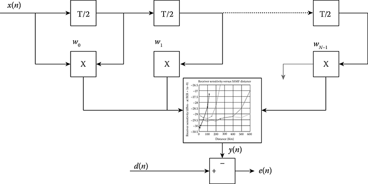
FIGURE 12.14 Structure of FIR filter for predistortion of the electrical driving signal at the optical transmitter.
sH(n)=[s*(n)..s*(n-1)..s*(n-2)...s*(n-N+1)]HsT(n)=[s(n)..s(n-1)..s(n-2)...s(n-N+1)]T(12.77)
and
cT=[c0..c1..c2...cN]TcH=[C*0..C*1C*2...C*N]H(12.78)
where the superscripts H and T denote the Hermitian and the transpose operation, respectively. The equalizer output can then be expressed in matrix form
y(n)=cTs(n)(12.79)
Note that the samples of the input s(n) and output y(n) of the equalizer are at T/2 intervals. However, in the optimization of the equalizer tap weights, only the output samples at T intervals are of concern. Thus, the error signal is defined as
e(n)=d(n)-y(2n)(12.80)
Figure 12.14 shows the proposed pre-equalization scheme and the fractionally spaced FIR filter, and thus the performance function to be minimized is written as
J=E[e2(n)]d(n)=∑iγjw(n-i)(12.81)
where γI is the impulse response of the digital duobinary filter. This impulse response, if under numerical simulation, would be padded with enough zeros to account for the delay of the transmitter filter and optical fiber, and is the uncorrupted data sequence. The fractionally sampled channel response (includes both the transmitter filter and optical fiber) is expressed as
y(nT)=[y0..y1..y2..yM-1]T(12.82)
where h is a sufficiently large integer such that the values of hi for i > (M−1) are negligible. The optimum tap weights are obtained by solving the Wiener–Hopf equation [3], which yields the optimum tap-weight vector, given by
c0 R−1p
with
R=E[s(2n)sH(2n)] and p=E[d*(n)s(2n)](12.83)
and
s(2n)=Hw(n)+v(2n)w(n)=[w(n)..w(n−1).....w(n−N2+1)]TwithH=[y0y2y4y6...yM−20...0y1y3y5...yM−3yM−1...00y2y4...yM−4yM−2...................]T(12.84)
w(n) is a vector of noise samples. Note that the matrix H is a circulant matrix with alternating rows in which a row is formed by shifting one column of the row to two levels above it. The noise, taken to be white noise, is added to avoid excessive filter gains at the frequencies where the magnitude of the channel frequency response is very small. Equation 12.14 may also be rewritten as
d(n)=γTw(n)(12.85)
where d(n) is a column vector of the target impulse response. From Equation 12.14, we can obtain
R=E[HssHHH]+σ2I=HIHH+σ2I=HHH+σ2I(12.86)
where σ is the variance of the added noise, and I is an identity matrix. Similarly
P=E[HwHHHγ]=HIγ+HIγ(12.87)
Thus, the desired optimum T/2-spaced FIR equalizer can be written as
c0=[HHH+σ2I]-1Hγ(12.88)
Figure 12.15 [13] shows significant improvement of the sensitivity of the linear equalizer in the 10 Gbps duobinary modulation format under the following conditions as shown in Table 12.3. Recently, the fundamental limits of the direct detection of duobinary modulation signals have been reported [7].

FIGURE 12.15 Receiver sensitivity versus fiber SSMF distance for conventional NRZ-ASK, NRZ duobinary, and predistortion equalized duobinary of different number of taps of the linear equalization system. (Adopted and simulation checked from N. Alic et al., Performance of maximum likelihood sequence estimation with different modulation formats, in Proceedings of LEOS’04, pp. 49–50, 2004.)
TABLE 12.3
Key Simulation Parameters Used in the LE for Duobinary Modulation Format

Eye opening penalty as a function of the dispersion tolerance in kms of SSMF under self-homodyne detection without and with linear equalizer FFE-DFE-NLC is shown in Figure 12.16.
12.5 MLSE Equalizer for Optical MSK Systems
12.5.1 Configuration of MLSE Equalizer in OFDR
Figure 12.17 shows the block diagram of narrowband filter receiver integrated with nonlinear equalizers for the detection of 40 Gbps optical MSK signals. Two narrowband filters are used to discriminate the USB and LSB frequencies that correspond to logic “1” and “0” transmitted, respectively. A constant optical delay line that is easily implemented in integrated optics is introduced on one branch to compensate for the differential group velocity delay td = 2π fd β2 L between F1 and F2, where fd = f1 − f2 = R/2, β2 represents group velocity delay (GVD) parameter of the fiber, and L is the fiber length. If the differential group delay is fully compensated, the optical lightwaves in two paths arrive at the photodiodes simultaneously. The outputs of the filters are then converted into the electrical domain through the photodiodes. These two separately detected electrical signals are sampled before being fed as inputs to the nonlinear equalizer.

FIGURE 12.16 Eye opening penalty as a function of the dispersion tolerance in kms of SSMF without and with linear equalizer FFE-DFE-NLC.

FIGURE 12.17 Block diagram of narrowband filter receiver integrated with nonlinear equalizers for the detection of 40 Gbps optical MSK signals.
12.5.2 MLSE Equalizer with Viterbi Algorithm
At epoch k, it is assumed that the effect of ISI on an output symbol of the finite state machine (FSM) ck is caused by both executive δ pre-cursor and δ post-cursor symbols on each side. First, a state trellis is constructed with 2δ states for both detection branches of the OFDR. A lookup table per branch corresponding to symbols “0” and “1” transmitted and containing all the possible 22δ states of all 11 symbol-length possible sequences is constructed by sending all the training sequences incremented from 1 to 22δ.
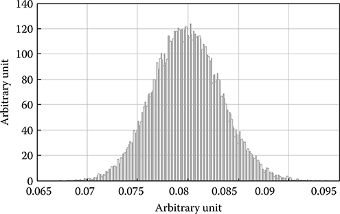
FIGURE 12.18 Noise distribution following Gaussian shape due to narrowband optical filtering.
The output sequence c(k) = f(bk, bk−1,…,bk−2δ−1) = (c1, c2,…,c2δ) is the nonlinear function representing the ISI caused by the δ adjacent pre-cursor and post-cursor symbols of the optical fiber FSM. This sequence is obtained by selecting the middle symbols ck of 2δ possible sequences with a length of 2δ + 1 symbol intervals.
The samples of the two filter outputs at epoch k yik, i = 1, 2 can be represented as yi(k)=ci(k)+niASE(k)+niElec(k), i = 1, 2. Here, niASE and niElec represent the amplified spontaneous emission (ASE) noise and the electrical noise, respectively.
In linear transmission of an optical system, the received sequence yn is corrupted by the ASE noise of the optical amplifiers, nASE, and the electronic noise of the receiver, nE. It has been proven that the calculation of branch metric and hence state metric is optimum when the distribution of noise follows the normal/Gaussian distribution—that is, the ASE noise and the electronic noise are collectively modeled as samples from Gaussian distributions. If noise distribution departs from the Gaussian distribution, the minimization process is suboptimum.
The Viterbi algorithm subsystem is implemented on each detection branch of the OFDR. However, the MLSE with Viterbi algorithm may be too computationally complex to be implemented at 40 Gbps with the current integration technology. However, there have been commercial products available for 10 Gbps optical systems. Thus, a second MLSE equalizer using the technique of reduced-state template matching is presented in the next section.
In an optical MSK transmission system, narrowband optical filtering plays the main role in shaping the noise distribution back to the Gaussian profile. The Gaussian-profile noise distribution is verified in Figure 12.18. Thus, branch metric calculation in the Viterbi algorithm, which is based on minimum Euclidean distance over the trellis, can achieve optimum performance. Also, the computational effort is less complex than ASK or DPSK systems due to the issue of non-Gaussian noise distribution.
12.5.3 MLSE Equalizer with Reduced-State Template Matching
The modified MLSE is a single-shot template-matching algorithm. First, a table of 22δ+1 templates, gk, k = 1, 2, …, 22δ+1, corresponding to the 22δ+1 possible information sequences, Ik of length 2δ + 1, is constructed. Each template is also a vector of size 2δ + 1, which is obtained by transmitting the corresponding information sequence through the optical channel and obtaining the 2δ + 1 consecutive received samples. At each symbol period, n the sequence, ˆIn with the minimum metric is selected as c(k)=arg minb(k) {m(b(k),y(k))}. The middle element of the selected information sequence is then output as the nth decision, În, that is, În = În(δ + 1). The minimization is performed over the information sequences, Ik, which satisfy the condition that the δ − 2 elements are equal to the previously decoded symbols În−δ, În−(δ−1), …, În−2 and the metric, m(Ik, rn), is given by m(Ik, rn) = {w·(gk − rn)}T{w·(gk − rn)}, where w is a weighting vector that is chosen carefully to improve the reliability of the metric. The weighting vector is selected so that, when the template is compared with the received samples, less weighting is given to the samples further away from the middle sample. For example, we found through numerical results that a weighting vector with elements w(i) = 2−|i−(δ+1)|, i = 1, 2, …, 2δ + 1 gives good results. Here, · represents Hadamard multiplication of two vectors, ( · )T represents transpose of a vector, and |·| is the modulus operation.
12.6 MLSE Scheme Performance
12.6.1 Performance of MLSE Schemes in 40 Gbps Transmission
Figure 12.19 shows the simulation system configuration used for the investigation of the performance of both the preceding schemes when used with the narrowband optical Gaussian filter receiver for the detection of noncoherent 40 Gbps optical MSK systems. The input power into fiber (P0) is −3 dBm, which is much lower than the nonlinear threshold power. The EDFA2 provides 23 dB gain to maintain the receiver sensitivity of −23.2 dBm at BER = 1e − 9. As shown in Figure 12.19, the optical received power (PRx) is measured at the input of the narrowband MSK receiver, and the OSNR is monitored to obtain the BER curves for different fiber lengths. The length of SSMF is varied from 48 to 60 km in steps of 4 km to investigate the performance of the equalizers to the degradation caused by fiber cumulative dispersion. The narrowband Gaussian filter with the time bandwidth product of 0.13 is used for the detection filters.
Electronic noise of the receiver can be modeled with equivalent noise current density of electrical amplifier of 20 pA/√Hz and dark current of 10 nA. The key parameters of the transmission system are given in Table 12.4.

FIGURE 12.19 Simulation setup for performance evaluation of MLSE and modified MLSE schemes for the detection of 40 Gbps optical MSK systems.
TABLE 12.4
Key Simulation Parameters Used in the MLSE-MSK Modulation Format
| Input power: P0 = −3 dBm | Narrowband Gaussian filter: B = 5.2 GHz or BT = 0.13 |
| Operating wavelength: λ = 1550 nm | Constant delay: td = |2πfDβ2L| |
| Bit rate: R = 40 Gbps | Preamp. EDFA of the OFDR: G = 15 dB and NF = 5 dB |
| SSMF fiber: |β2| = 2.68e−26 or |D| = 17 ps/nm/km | id = 10 nA |
| Attenuation: α = 0.2 dB/km | Neq = 20 pA/(Hz)1/2 |

FIGURE 12.20 Performance of modified Viterbi-MLSE and template-matching schemes, BER versus OSNR.
The Viterbi algorithm used with the MLSE equalizer has a constraint length of 6 (i.e., 25 number of states) and a trace-back length of 30. Figure 12.20 shows the BER performance of both nonlinear equalizers plotted against the required optical OSNR. The BER performance of the optical MSK receiver without any equalizers for 25 km SSMF transmission is also shown in Figure 12.20 for quantitative comparison. The numerical results are obtained via Monte Carlo simulation (triangular markers as shown in Figure 12.20) with the low BER tail of the curve linearly extrapolated.
The OSNR penalty (at BER = 1e − 9) versus residual dispersion corresponding to 48, 52, 56, and 60 km SSMF are presented in Figure 12.21. The MLSE scheme outperforms the modified MLSE schemes, especially at low OSNR. In the case of 60 km SSMF, the improvement at BER = 1e−9 is approximately 1 dB and, in the case of 48 km SSMF, the improvement is about 5 dB. In case of transmission of 52 km and 56 SSMF, MLSE with Viterbi algorithm has 4 dB gain in OSNR, compared to the modified scheme. With residual dispersion at 816, 884, 952, and 1020 ps/nm, at a BER of 1e−9, the MLSE scheme requires 12, 16, 19, and 26 dB OSNR penalty, respectively, while the modified scheme requires 17, 20, 23, and 27 dB OSNR, respectively.
12.6.2 Transmission of 10 Gbps Optical MSK Signals over 1472 km SSMF Uncompensated Optical Link
Figure 12.22 shows the simulation setup for 10 Gbps transmission of optical MSK signals over 1472 km SSMF. The receiver employs an optical narrowband frequency discrimination receiver integrated with a 1024-state Viterbi-MLSE postequalizer. The input power into the fiber (P0) is −3 dBm lower than the fiber nonlinear threshold power. The optical amplifier EDFA1 provides an optical gain to compensate the attenuation of each span completely. EDFA2 is used as a noise-loading source to vary the required OSNR. The receiver electronic noise is modeled with equivalent noise current density of the electrical amplifier of 20 pA/√Hz and dark current of 10 nA for each photodiode. A narrowband optical Gaussian filter with two-sided bandwidth of 2.6 GHz (one-sided BT = 0.13) is optimized for detection. A back-to-back OSNR = 8 dB is required for BER at 1e−3 for each branch. The correspondent received power is −25 dBm. This low OSNR is possible due to the large suppression of noise after being filtered by narrowband optical filters. A trace-back length of 70 is used in the Viterbi algorithm. Figure 12.22 shows the simulation results of BER versus the required OSNR for 10 Gbps optical MSK transmission over 1472 and 1520 km SSMF uncompen-sated optical links with one, two, and four samples per bit, respectively. The 1520 km SSMF with one sample per bit is seen as the limit for 1024-state Viterbi algorithm due to the slow roll-off and the error floor. However, two and four samples per bit can obtain error values lower than the FEC limit of 1e−3.
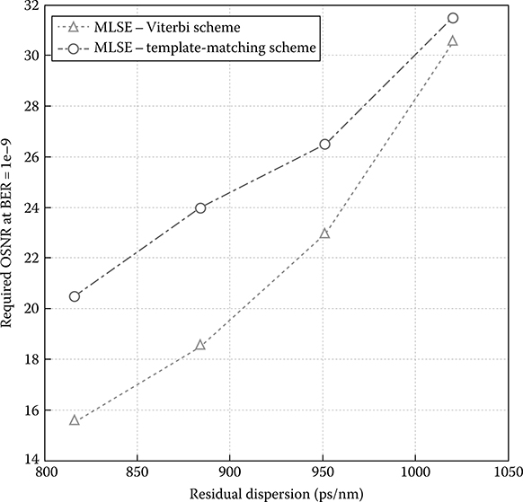
Figure 12.21 Required OSNR (at BER = 1e−9) versus residual dispersion in Viterbi-MLSE and template-matching MLSE schemes.
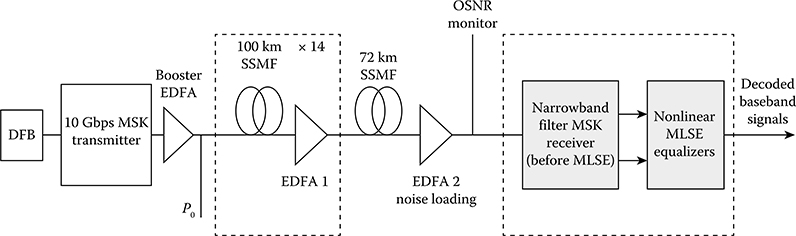
FIGURE 12.22 Simulation setup for transmission of 10 Gbps optical MSK signals over 1472 km SSMF with MLSE-Viterbi equalizer integrated with the narrowband optical filter receiver.

FIGURE 12.23 BER versus required OSNR for transmission of 10 Gbps optical MSK signals over 1472 and 1520 km SSMF uncompensated optical link.
Thus, 1520 km SSMF transmission of 10 Gbps optical MSK signals can reach error-free detection with the use of a high-performance FEC. In the case of 1472 km SSFM transmission, the error events follow a linear trend without sign of error floor and, therefore, error-free detection can be comfortably accomplished.
Figure 12.23 also shows the significant improvement in OSNR of two and four samples per bit over one sample per bit counterpart with values of approximately 5 and 6 dB, respectively. In terms of OSNR penalty at a BER of 1e−3 from back-to-back setup, four samples per bit for 1472 and 1520 km transmission distance suffers 2 and 5 dB penalty, respectively.
12.6.3 Performance Limits of Viterbi-MLSE Equalizers
The performance limits of Viterbi-MLSE equalizer to combat ISI effects are investigated against various SSMF lengths of the optical link. The number of states used in the equalizer is incremented according to this increase and varied from 26 to 210. This range was chosen as reflecting the current feasibility and future advance of electronic technologies that can support high-speed processing of the Viterbi algorithm in the MLSE equalizer. In addition, these numbers of states also provide feasible time for simulation.
In addition, one possible solution to ease the requirement of improving the performance of the equalizer without increasing much the complexity is by multisampling within one-bit period. This technique can be done by interleaving the samplers at different times. Although a greater number of electronic samplers are required, they only need to operate at the same bit rate as the received MSK electrical signals. Moreover, it will be shown later on that there is no noticeable improvement with more than two samples per bit period. Hence, the complexity of the MLSE equalizer can be affordable while improving the performance significantly.
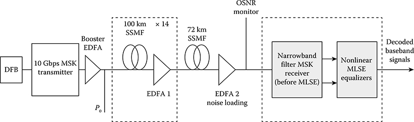
FIGURE 12.24 Simulation setup of OFDR-based 10 Gbps MSK optical transmission for the study of performance limits of the Viterbi-MLSE equalizer.
Figure 12.24 shows the simulation setup for 10 Gbps optical MSK transmission systems with lengths of uncompensated optical links varying up to 1472 km SSMF. In this setup, the input power into fiber (P0) is set to be −3 dBm, thus avoiding the effects of fiber nonlinearities. The optical amplifier EDFA1 provides an optical gain to compensate for the attenuation of each span completely. The EDFA2 is used as a noise-loading source to vary the required OSNR values. Moreover, a Gaussian filter with two-sided 3-dB bandwidth of 9 GHz (one-sided BT = 0.45) is utilized as the optical discrimination filter because this BT product gives the maximized detection’s eye openings (refer to Section 9.4). The receiver’s electronic noise is modeled with equivalent noise current density of the electrical amplifier of 20 pA/√Hz and a dark current of 10 nA for each photodiode. A back-to-back OSNR = 15 dB is required for a BER of 1e−4 on each branch, and the corresponding receiver sensitivity is −25 dBm. A trace-back length of 70 is used for the Viterbi algorithm in the MLSE equalizer. Figures 12.24 through 12.26 show the BER performance curves of 10 Gbps OFDR-based MSK optical transmission systems over 928, 960, 1,280, and 1470 km SSMF uncompensated optical links for different numbers of states used in the Viterbi-MLSE equalizer. In these figures, the performance of Viterbi-MLSE equalizers is given by the plot of the BER versus the required OSNR for several detection configurations: balanced receiver (without the equalizer), the conventional single-sample-per-bit sampling technique, and the multisample-per-bit sampling techniques (two and four samples per bit slot). The simulation results are obtained by the Monte Carlo method.
The significance of multisamples per bit slot in improving the performance for MLSE equalizer in cases of uncompensated long distances is shown. It is found that the tolerance limits to the ISI effects induced from the residual CD of a 10 Gbps MLSE equalizer using 26, 28, and 210 states are approximately equivalent to lengths of 928, 1280, and 1440 km SSMF, respectively. The equivalent numerical figures in the case of 40 Gbps transmission correspond to lengths of 62, 80, and 90 km SSMF, respectively.
In the case of 64 states over 960 km SSMF uncompensated optical link, the BER curve encounters an error floor that cannot be overcome even by using high-performance FEC schemes. However, at 928 km, the linear BER curve indicates the possibility of recovering the transmitted data with the use of a high-performance FEC. Thus, for 10 Gbps OFDR-based MSK optical systems, a length of 928 km SSMF can be considered as the transmission limit for the 64-state Viterbi-MLSE equalizer. Results shown in Figure 12.26 suggest that the length of 1280 km SSMF uncompensated optical link is the transmission limit for the 256-state Viterbi-MLSE equalizer when incorporating with OFDR optical front end. It should be noted that this is achieved when using the multisample-per-bit sampling schemes.
It is observed from Figure 12.27 that the transmission length of 1520 km SSMF with one sample per bit is seen as the limit for the 1024-state Viterbi algorithm due to the slow roll-off and the error floor. However, two and four samples per bit can obtain error values lower than the FEC limit of 1e−3. Thus, 1520 km SSMF transmission of 10 Gbps optical MSK signals can reach error-free detection with the use of a high-performance FEC. In case of 1472 km SSFM transmission, the error events follow a linear trend without the sign of error floor and, therefore, error-free detection can be achieved. Figure 12.27 also shows the significant OSNR improvement of the sampling techniques with two and four samples per bit compared to the single-sample-per-bit counterpart. In terms of OSNR penalty at BER of 1e−3 from back-to-back setup, four samples per bit for 1472 and 1,520 km transmission distance suffers 2 and 5 dB penalty, respectively.

FIGURE 12.25 Performance of 64-state Viterbi-MLSE equalizers for 10 Gbps OFDR-based MSK optical systems over (a) 960 km and (b) 928 km SSMF uncompensated links.

FIGURE 12.26 Performance of 256-state Viterbi-MLSE equalizer for 10 Gbps OFDR-based MSK optical systems over 1280 km SSMF uncompensated link.
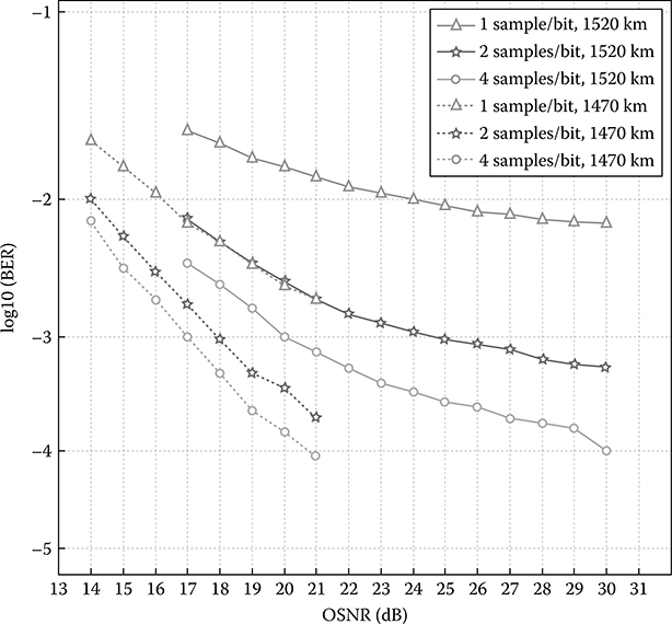
FIGURE 12.27 Performance of 1024-state MLSE equalizer for 10 Gbps optical MSK signals versus required OSNR over 1472 and 1520 km SSMF uncompensated optical link.
It is found that, for incoherent detection of optical MSK signals based on the OFDR, an MLSE equalizer using 24 states does not offer better performance than the balanced configuration of the OFDR itself, that is, the uncompensated distance is not over 35 km SSMF for 40 Gbps or 560 km SSMF for 10 Gbps transmission systems, respectively. It is most likely that, in this case, the severe ISI effect caused by the optical fiber channel has spread beyond the time window of five bit slots (two pre-cursor and two post-cursor bits), the window that 16-state MLSE equalizer can handle.
The trace-back length used in the investigation is chosen to be 70, which guarantees the convergence of the Viterbi algorithm. The longer the trace-back length, the larger the memory that is required. With the state-of-the-art technology for high storage capacity nowadays, memory is no longer a big issue. Very fast processing speed at 40 Gbps operations hinders the implementation of 40 Gbps Viterbi-MLSE equalizers at the mean time. Multisample sampling schemes offer an exciting solution for implementing fast signal processing algorithms. This challenge may also be overcome in the near future together with the advance of the semiconductor industry. At the present, the realization of Viterbi-MLSE equalizers operating at 10 Gbps has been commercially demonstrated [14].
12.6.4 Viterbi-MLSE Equalizers for PMD Mitigation
Figure 12.28 shows the simulation test bed for the investigation of MLSE equalization of the PMD effect. The transmission link consists of a number of spans that comprise 100 km SSMF (with D = +17 ps/(nm·km), α = 0.2 dB/km) and 10 km DCF (with D = −170 ps/(nm·km), α = 0.9 dB/km). Input power into each span (P0) is −3 dBm. The EDFA1 has a gain of 19 dB, hence providing input power into the DCF to be −4 dBm, which is lower than the nonlinear threshold of the DCF. The 10 dB gain of EDFA2 guarantees the input power into next span unchanged of −3 dBm value. An OSNR of 10 dB is required for receiver sensitivity at BER of 1e−4 in case of back-to-back configuration. Considering the practical aspect and complexity a Viterbi-MLSE equalizer for PMD equalization, a small number of four state bits, or effectively 16 states, were chosen for the Viterbi algorithm in the simulation study.
The performance of MLSE against the PMD dynamic of optical fiber is investigated. BER versus required OSNR for different values of normalized average differential group delay (DGD) <Δτ> are shown in Figure 12.29. The mean DGD factor is normalized over one-bit period of 100 and 25 ps for 10 and 40 Gbps bit rate, respectively. The numerical studies are conducted for a range of values from 0 to 1 of normalized DGD <Δτ>, which equivalently corresponds to the instant delays of up to 25 or 100 ps in terms of 40 and 10 Gbps transmission bit rate, respectively.
The advantages of using multiple samples per bit over the conventional single sample per bit in MLSE equalizers are also numerically studied, and the Monte Carlo results for normalized DGD values of 0.38 and 0.56 are shown in Figures 12.30 and 12.31. However, the increase from two to four samples per bit does not offer any gain in the performance of the Viterbi-MLSE equalizer. Thus, two samples per bit are preferred to reduce the complexity of the equalizer. Here, and for the rest of this chapter, multisamples per bit implies the implementation of two samples per bit. Performance of MLSE equalizer for different normalized DGD values with two samples per bit is shown in Figure 12.32. From Figure 12.32, the important remark is that 16-state MLSE equalizer implementing two samples per bit enables the optical MSK transmission systems achieving a PMD tolerance of up to one-bit period at BER = 1e−4 with a required OSNR of 8 dB. This delay value starts introducing a BER floor indicating the limit of the 16-state MLSE equalizer. This problem can be overcome with a high-performance FEC. However, the DGD mean value of 0.94 can be considered as the limit for an acceptable performance of the proposed MLSE equalizer without the aid of a high-performance FEC. Figure 12.33 shows the required OSNR for MLSE performance at 1e−4 versus normalized <Δτ> values in configurations of balanced receiver, one sample per bit, and two samples per bit.
A balanced receiver without the use of the MLSE equalizer requires an OSNR = 5 dB to obtain a BER = 1e−4 when there is no effect of the PMD at all compared to the required OSNR of 3 dB and 1 dB in cases of one sample per bit and two samples per bit. The OSNR penalties for various normalized <Δτ> values for the preceding three configurations are shown in Figure 12.34.

FIGURE 12.28 Simulation test bed for investigation of effectiveness of MLSE equalizer to PMD.
It can be observed that the OSNR penalties (back-to-back) of approximately 3 and 1 dB apply to the cases of balanced receiver and one sample per bit, respectively, with reference to the two-samples-per-bit configuration. Another important remark is that the 16-state Viterbi-MLSE equalizer that implements two samples per bit enables the optical MSK transmission systems to achieve a PMD tolerance of up to one-bit period at a BER of 1e−4 with a power penalty of about 6 dB. Moreover, the best 2 dB penalty occurs at 0.75 for the value of normalized <Δτ>. This result shows that the combination of OFDR-based MSK optical systems and Viterbi-MLSE equalizers, particularly with the use of multisample sampling schemes, was found to be highly effective in combating the fiber PMD dynamic impairment and better than the recently reported PMD performance for OOK and DPSK modulation formats [15].
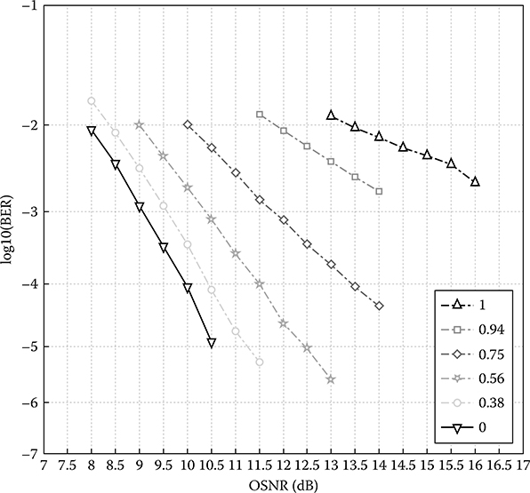
FIGURE 12.29 Performance of MLSE equalizer versus normalized <Δτ> values for one sample per bit.

FIGURE 12.30 Comparison of MLSE performance for configurations of one, two, and four samples per bit with normalized <Δτ> value of 0.38.

FIGURE 12.31 Performance of Viterbi-MLSE equalizer for configurations of one, two, and four samples per bit with a normalized <Δτ> value of 0.56.

FIGURE 12.32 Performance of Viterbi-MLSE equalizer for different normalized <Δτ> values with two and four samples per bit.
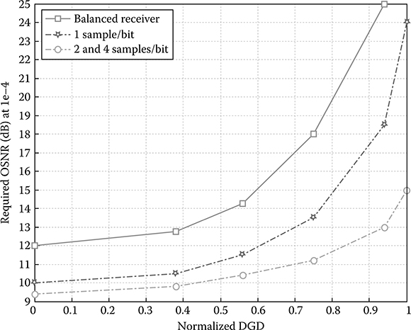
FIGURE 12.33 Required OSNR for MLSE performance at 1e−4 versus normalized <Δτ> values in configurations of balanced receiver and one and two samples per bit.
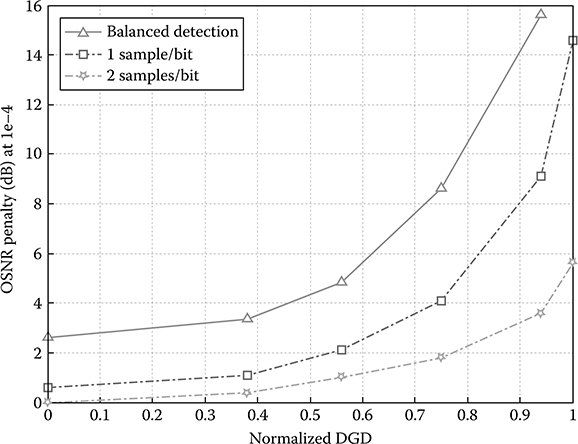
FIGURE 12.34 OSNR penalties of MLSE performance at 1e−4 for various normalized <Δτ> values in configurations of balanced receiver, single-sample, and two-samples-per-bit sampling schemes.
12.6.5 The Uncertainty and Transmission Limitation of the Equalization Process
The fundamental limitations of a quadratic phase media on the transmission speed are formulated in signal space for significant applications in signal equalization. These limitations are quantitatively derived for both coherent and incoherent optical systems. This section investigates the dispersive effect of optical fiber on the transmission speed of the media. The main effect of dispersion is pulse broadening (and frequency chirping), as the signal pulses propagate through the quadratic phase media. This causes ISI, thereby limiting the speed of transmission. There are various ways of mitigating the harmful effects of ISI. One way is to use optical fiber with anti-dispersive property to equalize the dispersion. In practice, this optical scheme reduces the signal level, and thus requires amplification. The amplifier introduces noise, which in turn limits the channel speed (Shannon’s information capacity theorem). Another way of combating ISI is by digital electronic equalization means such as MLSE, which is applicable for both coherent and incoherent detection schemes [13,15,16,17 and 18]. These reported results show clearly that there is a fundamental limit on the achievable transmission speed for a given fiber length.
This section studies the limitations of the quadratic phase channel, the single-mode optical fiber, in terms of signal space. The signal space is chosen so that it consists of binary signals in an 8-bit block code. As the eight-bit symbols propagate down the quadratic phase channel, the waveform patterns of the symbols would naturally become less and less distinctive, hence making it more and more difficult to discriminate between the symbols. How do we quantify the detrimental effect of the quadratic phase channel? It is obvious that the more information we have at hand, the more accurate one would be able to obtain the BER. We approach this problem entirely from a digital communications perspective, and the results so derived are the fundamental limit imposed by the quadratic phase channel. It is virtually independent of the detection scheme used. Two mechanisms that limit the transmission speed are explained. One is brought about by the finite time window available for detection. In all practical schemes, the decoder must decode each symbol within a finite period of time. The other is brought about by not using the phase information for detection. Depending on the complexity of the detection scheme chosen, the phase information is quite often lost inadvertently when the optical signal is converted into the electrical signal.
12.7 Nonlinear MLSE Equalizers for MSK Optical Transmission Systems
12.7.1 Nonlinear MLSE
MLSE is a well-known technique in communications for the equalization and detection of the transmitted digital signals. The concept of MLSE is discussed in brief here. An MLSE receiver determines a sequence b as the most likely transmitted sequence when the conditional probability Pr(y|b) is maximized, where y is the received output sequence. If the received signal y is corrupted by a noise vector n that is modeled as a Gaussian source (i.e., y = b + n), it is shown that the preceding maximization operation can be equivalent to the process of minimization of the Euclidean distance d4
d=∑k|yk-bk|2(12.89)
MLSE can be carried out effectively with the implementation of the Viterbi algorithm based on state trellis structure.
12.7.2 Trellis Structure and Viterbi Algorithm
12.7.2.1 Trellis Structure
Information signal b is mapped to a state trellis structure by an FSM, giving the mapping output signal c as shown in Figure 12.35. The FSM can be a convolutional encoder, a trellis-based detector, or, as presented in more detail later on, the fiber medium for optical communications.
A state trellis structure created by the FSM is illustrated in Figure 12.36. At the epoch nth, the current state B has two possible output branches connecting to states E and F. In this case, these two branches correspond to the two possible transmitted symbols of “0” or “1,” respectively. This predefined state trellis applies to the one bit per symbol modulation formats such as binary ASK or DPSK formats. In cases of multibit modulation per symbol, the phase trellis has to be modified. For example, in the case of DQPSK, there are four possible branches leaving the current state B and connecting the next states, corresponding to the possible input symbols of “00,” “01,” “10,” and “11.”
Furthermore, for a simplified explanation, several assumptions are made. These assumptions and according notations can be described as follows.
Current state B is the starting state of only two branches that connect to states E and F, denoted as bBE and bBF. In general, bB* represents all the possible branches in the trellis that starts from state B. In this case, these two branches correspond to the possible binary transmitted information symbols of “0” or “1,” respectively. The notation c(B,a = 0) represents the encoded symbol (at the FSM output) for the branch BE, bBE, which starts from state B and corresponds to a transmitted symbol a = 0. Similar conventions are applied for the case of branch BF, bBF, that is, c(B,a = 1), and the all the branches in the trellis.

FIGURE 12.35 Schematic of the MLSE equalizer as a finite state machine (FSM).

FIGURE 12.36 State trellis of an FSM: (a) trellis path and (b) tracing of possible maximum-likelihood estimation with assigned bit pattern.
There are only two possible output branches ending at state E (from state A and state B). They are denoted as bAE and bBF. In general, b*E represents all the possible branches in the trellis that end at state E. The number of states 2δ in the trellis structure is determined by the number of memory bits, δ, also known as the constraint length. Figure 12.36b also shows a possible trace of the trellis with the assigned states of the bit pattern.
12.7.2.2 Viterbi Algorithm
The principles of the Viterbi algorithm follow two principal stages as follows:
12.7.2.2.1 Calculation of State and Branch Metrics
At a sampling index n, epoch n, a branch metric is calculated for each of the branches in the trellis. For example, considering the connecting branch between the current state B and the next state E, which corresponds to the case when the “0” symbol is transmitted, the branch metric BMBE is calculated as BMBE(n) = |y(n)−cBE|2.
The state metric SME(n) of the state E is calculated as the sum between the metric of the previous state, that is, state B and the branch metric obtained earlier. The calculation of state metric SME(n) of state E is given by
SME(n)=min∀B→E{SMB(n-1)+BMBE(n)}(12.90)
The branch giving the minimum state metric SME(n) for state E is named as the preferred path.
12.7.2.2.2 Trace-Back Process
The process of calculating state and branch metrics continues along the state trellis before terminating at epoch Ntrace, which is usually referred to as the trace-back length. A rule of thumb, as shown in Refs. [19,20], is that the value of Ntrace is normally taken to be five times the sequence length. This value comes from the results showing that the solution for the Viterbi algorithm converges, giving a unique path from epoch 1 to epoch Ntrace for the MLSE detection. (1) At Ntrace, the terminating state with the minimum state metric and its connecting preferred path are identified. (2) The previous state is then identified, as well as its previous preferred path. (3) The trace-back process continues until reaching epoch 1.
12.7.3 Optical Fiber as an FSM
The FSM shown in Figure 12.36 is now replaced with the optical channel based on optical fibers. It is significant to understand how the state trellis structure is formed for an optical transmission system. In this case, the optical fiber involves all the ISI sources causing the waveform distortion of the optical signals, which includes CD, PMD, and filtering effects. Thus, the optical fiber FSM excludes the signal corruption by noise as well as the random-process nonlinearities. The ISI caused by dispersion phenomena and nonlinear phase and ASE and nonlinear effects has been described in Chapters 3 and 8.
The construction of state trellis structure can be implemented in the following. At epoch n, it is assumed that the effect of ISI on an output symbol of the FSM cn is caused by both executive δ pre-cursor and δ post-cursor symbols on each side. In this case, cn is the middle symbol of a sequence that can be represented as c = (Cn–δ,..., Cn,..., Cn+δ) b ∈ {0,1}; n > 2δ + 1. Unlike the conventional FSM used in wireless communications, the output symbol cn of the optical fiber FSM is selected as the middle symbol of the sequence c. This is due to the fact that the middle symbol gives the most reliable picture about the effects of ISI in optical fiber channels.
A state trellis is defined with a total number of 22δ possible data sequences. At epoch n, the current state B is determined by the data sequence (bn–2δ + 1,...,bn–δ,...bn) b∈{0,1}; n ≥ 2δ + 1, where bn is the current input symbol into the optical fiber FSM. Therefore, the state trellis structure can be constructed from the optical fiber FSM, and is ready to be integrated with the Viterbi algorithm, especially for the calculation of a branch metric.
The MLSE nonlinear equalizer can effectively combat all the preceding ISI effects, and it is expected that the tolerance to both CD and PMD of optical MSK systems with an OFDR receiver can be improved significantly.
12.8 Uncertainties in Optical Signal Transmission
12.8.1 Uncertainty in ASK Modulation Optical Receiver without Equalization
There are many ways of coding the data for transmission through the optical fiber. For simplicity, we first choose an NRZ-ASK system for this study, and the transmission rate is operating at 40 Gbps. Later in this section, we investigate the uncertainty of data recovery under MSK modulation and the use of equalization technique, and the MLSE in long-haul optically amplified transmission system.
The NRZ-ASK transmitted signal is organized into eight-bit blocks, and, thus, there are 28 (256) possible pattern symbols. As the eight-bit symbols propagate down the quadratic phase channel, the waveform patterns of the symbols would become less and less distinctive. It makes the task of decoding more and more difficult and uncertain. How do we measure this uncertainty? In the field of digital communications, the uncertainty of MLSE detection is measured in symbol error rate (SER), which is a function of the SNR. SNR, in turn, depends on the distances between signal constellation, and it is the shortest distance that dominates the error probability. The SER and the Q factor are expressed as a function of the normalized shortest Euclidean distance metric dnorm between all possible received symbol pair combinations as
SER=Q(√SNR)=Q(√d2norm×SNRnofiber)0<dnorm≤1(12.91)
where SNRnofiber is the optical SNR (OSNR) in the case of a back-to-back setup, that is, without fiber. From Equation 12.91, the logarithmic scale of d2norm represents the OSNR penalty as expressed in the following equation
d2norm[dB]=OSNR penalty=SNR[dB]−SNRnorfiber[dB](12.92)
Figure 12.37 depicts the penalty in the discrimination property, with the OSNR penalty being plotted against the length of the SSMF (the dispersion factor D = 17 ps/(nm·km)) for the case of coherent detection schemes, that is, both the magnitude and phase information of the received waveform are used.
The family of curves shown in Figure 12.37 corresponds to a range of different detection window widths; from a window of eight-bit periods (the minimum detection width) to 9-, 10-, and 32-bit periods. As expected, the discrimination property is significantly improved as the detection window length increases. In the case of 32-bit window length, there is insignificant penalty over the fiber lengths of up to 50 km SSMF. This result reaffirms the previous discussion that the channel capacity is infinite, that is, there is no uncertainty if the detection time window is long enough. At the fiber distance of 5 km, a penalty of about 0.7 dB occurs if the eight-symbol detection width is used. Depending on the system noise level, this signal level may or may not be acceptable for a reliable data transmission.
We are now considering incoherent optical transmission systems that utilize a photodiode to convert the optical signals to electrical signals. The use of photodiodes as such could result in the loss of the phase information of the signal. Furthermore, electrical equalization techniques based on the MLSE principles employ only the magnitude information [17, 12.42–12.44]. To model this incoherent property, the distance metric utilizes the absolute magnitude of the received waveform only. The discrimination penalty versus the length of SSMF is depicted in Figure 12.38.
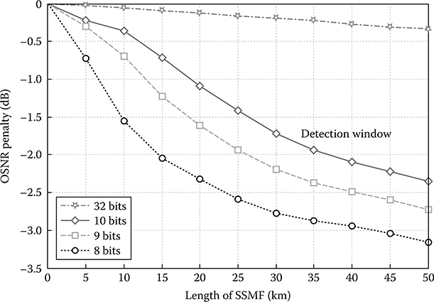
FIGURE 12.37 Discrimination penalty versus transmission distance at 40 Gbps when using both magnitude and phase information.

FIGURE 12.38 Discrimination penalty versus transmission distance at 40 Gbps when considering only the magnitude information.
The family of curves in Figure 12.38 also corresponds to a range of different detection window widths (8-, 9-, 10-, and 32-bit periods). When the length of the fiber is less than about 15 km, there is no appreciable improvement by choosing a larger detection window. However, when the length of the fiber increases further, the deterioration is quite severe, and having a larger detection window helps enormously in reducing this deterioration. At the SSMF length of 5 km, the incoherent detection suffers a penalty of approximately 3.5 dB, compared to the 0.7 dB penalty for the coherent detection, and, thus, leading to an improvement of about 3 dB when using the coherent schemes with the availability of both amplitude and phase information. This agrees with the popularly known advantage on the receiver sensitivity of coherent detections over the incoherent counterparts. In addition, comparing the two sets of results in Figures 12.37 and 12.38 shows clearly the extent of improvements possible if the coherent scheme is used instead of the incoherent scheme. This is achieved at the expense of greater system complexity on the receiver structure of coherent optical systems.
12.8.2 Uncertainty in MSK Optical Receiver with Equalization
The equalization processing system is placed at the output of the optical receiver shown in Figure 12.28, that is, the equalization is completed in the electronic domain, which means the optical impulse and pulses have been converted into the electrical domain and the phase chirping has already converted to amplitude distortion. However, the broadening of the pulse influences the sampled values obtained from the broadened pulses for the processing of the equalization system.
The narrowband filter receiver in Figure 12.35 is now integrated with the MLSE nonlinear equalizers for the detection of 40 Gbps optical MSK signals. Two narrowband filters are used to discriminate the USB and LSB frequencies that correspond to the logical “1” and “0” transmitted, respectively. A constant optical delay line that is easily implemented in integrated optics is introduced on one branch to compensate for the differential group delay td = 2πfdβ2L between the “1” and “0” logic pulses of frequencies F1 and F2, where fd = f1 − f2 = R/2, β2 represents the GVD parameter of the fiber, and L is the fiber length. If the differential group delay is fully compensated, the optical lightwaves in two paths arrive at the photodiodes simultaneously. The outputs of the filters are then converted into the electrical domain through the photodiodes. These two separately detected electrical signals are sampled before being fed as the inputs to the nonlinear equalizer. The MLSE equalizer requires values of the samples that occurred in advance as well as in later events. This is the impact of the impulse response of the fiber on this equalization, and the number of events required for the detection and equalization is very critical. Figure 12.27 shows the performance of the optical frequency discrimination integrated with an MLSE equalizer in a long-haul optically amplified fiber transmission system of about 1500 km when the number of one, two, and four samples per bit is used in the equalization processing system. The time distance between the samples is controlled, so that they are within the reasonable time slot under the effects of chirping of the phase of the lightwave.
12.9 Electronic Dispersion Compensation of Modulation Formats
Except the MLSE as the pattern comparison, and the decision made based on the matching, the equalization techniques using FFE, FFE-DFE, nonlinear equalization, and FFE result in different improvements of the eye opening of digital modulation formats of either amplitude shift keying of phase shift keying.
Simulations are conducted for NRZ formats with the modulation of ASK, DuoBinary, DPSK, and SSB. The transmission link setup is implemented with spans of non-CD compensating optically amplified fibers. The bit rate is 10 Gbps, and an optical filter of 50 GHz 3 dB passband is used before the optoelectronic detection. Transmission fibers are SSMF, and 17 ps/nm/km dispersion factor is assumed. The OSNR is plotted against the linear dispersion factor, as shown in Figures 12.39 through 12.42 for NRZ-ASK, NRZ duobinary (50%), NRZ-DPSK, and NRZ-SSB formats. It noted (1) moderate improvement of the OSNR for NRZ-ASK (Figure 12.39), (2) significant improvement of OSNR for the SSB format (see Figure 12.42), (3) mild improvement for the DPSK format, and (4) moderate improvement of the duobinary format.
Thus, effectively, we note that significant improvement of the eye opening is achieved for single-sideband signals. Why this is so? In order to explain these results, see recent clarifications by Rosenkranz and Xia [21], although attempts have also been made some years ago [22]. The behavior of the signals received after the photodetector, a square law detection device, can be explained using the phasor representation given in Figure 12.43 as follows.

FIGURE 12.39 OSNR required for BER 5e−4 (Monte Carlo simulation) versus linear CD under different equalization schemes for NRZ-ASK modulation format.

FIGURE 12.40 OSNR required for BER 5e−4 (Monte Carlo simulation) versus linear CD under different equalization schemes for NRZ duobinary modulation format.
Considering a monochromatic wave of frequency ω1 of the double sideband of the NRZ-ASK modulated carrier, then, under ASK modulation, the complex field envelope of the received signals entering the photodetector is given by
sASK(t)=1+Am2ej(ω1t-ϕA)+Bm2ej(-ω1t-ϕB)(12.93)
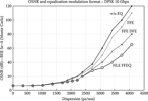
FIGURE 12.41 OSNR required for BER 5e−4 (Monte Carlo simulation) versus linear CD under different equalization schemes for NRZ-DPSK modulation format.

FIGURE 12.42 OSNR required for BER 5e−4 (Monte Carlo simulation) versus linear CD under different equalization schemes for NRZ-SSB modulation format.
The first term represents the carrier term at DC after the detection, the second and third terms come from the upper sideband (USB) and lower sideband (LSB), respectively, and m is the modulation index. The coefficients A and B and the additional phase shifts ϕA and ϕB are given by
A=|H(ω1)|=B=|H(-ω1)(12.94)
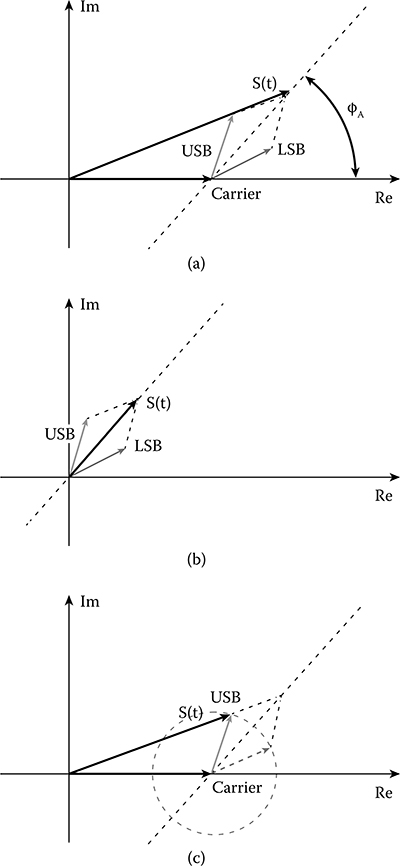
FIGURE 12.43 Phasor representation of optical signals under different modulation formats: (a) ASK—with carrier suppression and lower sideband (LSB) and upper sideband (USB), (b) SSB without carrier suppression, and (c) SSB with carrier suppressed plus USB.
where H(ω) = exp(−jβ2ω2), ϕA = ϕB = β2ω12L/2, with H(ω) being the fiber transfer function in the frequency domain. Thus, the electronic current generated by the photodetector is given by the squaring of the magnitude of the optical field, and can be written as
|sASK(t)|2=|1+Am2ej(ω1t-ϕA)+Bm2ej(-ω1t-ϕB)|2=1+m22+2mcosϕAcosω1t+m22cos2ω1t(12.95)
We note from this equation that there are three terms: a DC term, a first harmonic term (linear term), and a second harmonic term that represents the distortion due to dispersion.
In the case of the DPSK, duobinary, and SSB modulation formats, we can follow a similar analysis to obtain the electronic currents generated after the photodetector
|sDuoB(t)|2=|sDuoB(t)|2=m22(1+2m cosω1t)|sSSB(t)|2=1+m24+mcos(ω1t-ϕA)(12.96)
Obviously, the currents are linear, and no nonlinear term existed. A linear equalizer equalizes the signal waveform by minimizing the ISI due to the linear part of Equations 12.95 and 12.96. When the phase term cos(ϕA) becomes smaller after a propagation length of about 100 km (or 1700 ps/nm), the linear term diminishes significantly, and the linear equalization would have no effect. The nonlinear distortion term becomes significant and takes over the linear term, as we can observe from Figure 12.39.
It is noted that the linear part comes from the carrier component, whereas for DPSK and duo-binary, the carrier is embedded into the signal band and plays no role. As mentioned earlier, this is due to the effective sampling of the waveform by the switching on and off of the amplitude in ASK. Thus, from Equation 12.96, the linear term disappears, and hence the linear equalizer is not effective, as observed from Figures 12.40 and 12.41.
For SSB modulation, we could see that there is a DC term and a linear part. Thus, the linear FFE would perform well and compatible to that by the nonlinear FFE and DFE algorithms as observed in Figure 12.42.

FIGURE 12.44 Spectral illustration of DSB and SSB operation after the lightwave-modulated signals propagating through a fiber length.
We can visualize the effects of pure phase distortion channel on modulation schemes with DSB and SSB, as shown in Figure 12.44. For DSB modulation, the spectrum shown in Figure 12.44a in the baseband is shifted to the passband (Figure 12.44b). After propagating through the fiber, the spectrum amplitude remains the same, but its phase is altered by the fiber phase distortion by an amount –β2Lf2.
Hence, when the signals are recovered in the photodetector, the double sidebands interfere with each other, with the overlapping (hatched area) as shown in Figure 12.44c. Thus, distortion is generated by both the band distortion and the interference between the two sidebands. On the contrary, for SSB, this recovered process would not result in any interference. Hence, distortion could only come from the pure distortion within the bands, and no distortion would be due to spectral overlapping. Thus, linear equalization works well for SSB linear distortion.
12.10 Concluding Remarks
We have described the equalization of real and imaginary signals using FFE, DFE, and FFE, and linear and nonlinear equalizers that are placed at either the transmitters, the receivers, or shared between the receivers and transmitters. The effects of equalizers on modulation formats are identified.
For phase shift keying and duobinary, the carrier is embedded within the signal band, and hence there is only nonlinear frequency doubling terms that exist in the electronic current generated by the photodetector, and thus nonlinear equalization works well and linear FFE contributes no effect when the linear term diminishes after a certain length of the fiber. The electronic current generated under the SSB modulation format, on the other hand, exhibits only the linear term and no frequency doubling term (no nonlinear term), and thus the linear equalizer FFE works as well as the nonlinear equalizer. Thus, only FFE is required as the implementation of the FFE is much simpler at high speeds. We thus expect that linear FFE also works well for MSK modulation formats.
Supplementing these investigations to prove the effects of the carrier in modulation formats, two case studies have been conducted in detail. First, a study of a linear electrical equalizer for duobinary modulation formats has been conducted, and two nonlinear equalizers are proposed, MLSE using the Viterbi algorithm and the modified MLSE scheme, which are integrated with the narrowband optical filter receiver proposed in Refs. [15,23,24 and 25] for noncoherent detection of 40 Gbps optical MSK signals. This chapter has presented the nonlinear MLSE equalizers, especially when integrated with the Viterbi algorithm, for digital photonic communications in general and for OFDR-based MSK optical systems. The backgrounds of MSLE and the Viterbi algorithm are briefly given, and the construction of the state trellis structure for use in optical communications has been explained. It has also been shown that noise after tight optical filtering that follows the Gaussian distribution can be minimized. Thus, the Viterbi algorithm can obtain its optimum performance without requiring more complex algorithms for estimating the exact noise distribution. Two MLSE electronic equalizers based on Viterbi procedures and template-matching algorithms are investigated and formulated for OFDR-based MSK optical transmission systems. In these two schemes, OFDR serves as the optical front end. The proposed equalizers significantly extend the reach of uncompensated links. With a reasonably small number of states (64 states), the uncompen-sated optical link can equivalently reach up to approximately 960 km SSMF for 10 Gbps transmission or 60 km SSMF for 40 Gbps. The results are comparable to the distance of 1040 km SSMF, as reported previously [26] for OOK/IM systems, in which up to 8192 trellis states are required.
The performance of the Viterbi-MLSE equalizers for OFDR-based optical MSK transmission systems in terms of transmission limits and PMD mitigation was also numerically investigated. Finally, this chapter has proven the improvement in performance of Viterbi-MLSE equalizers by using multisamples per bit compared to the conventional single sample bit. The novel scheme in which Viterbi-MLSE equalizers are incorporated with OFDR-based MSK optical transmission systems provides high robustness to the fiber PMD dynamic and better performance compared to other modulation formats.
Finally, we investigated quantitatively the transmission limits due to the combination of the dispersive effect of the quadratic phase media and restrictiveness of a finite detection and equalization window. The parameter used to quantify these limits is the least Euclidian distance between all symbol combinations, and this distance corresponds to the penalty in the system’s OSNR. For the coherent detection, both phase and magnitude information of the received signals is used in the determination of the Euclidian distance, whereas only the magnitude information is used in the incoherent detection. It is found that coherent systems provide a much higher degree of discrimination, which is significant for the signal equalization at the cost of the receiver’s complexity.
There is no doubt that the equalizers must be adaptive for automatic control of the adjustment of the equalization due to the nature of the dispersion fluctuation of CD and PMD, as well as the nonlinear effects of signals transmitted over the long-haul distance. In practice, the equalizers described in this chapter must be adaptive. One such example is the equalization of channels that have been propagated through different hops of DWDM optical networks.
Electronic equalization emerges as an important technique for the mitigation of impairments of optical signals propagating through optical channels, and will remain a very probable candidate for reshaping the distorted signals. The progresses in the development of high-speed digital electronic processors will assist in the practical implementation of these equalizers in optical transmission systems and networks.
Ref. [22] has reported the electrical equalization of OFDM signals over long-haul transmission. The integration of multicarrier modulation and electrical equalization techniques would enable the extension of transmission beyond the dispersion limit in single-mode optical fiber communications systems. However, the double-sideband modulation of OFDM to the optical passband may face nonlinearity distortion, and the equalizer may have to be nonlinear, causing difficulties in the implementation, unless it is implemented after the recovery of the bit sequence after the PFDM decoder, as described in Chapter 11.
References
1. Y. Matsui, D. Mahgerefteh, X. Zheng, C. Liao, Z. F. Fan, K. McCallion, and P. Tayebati, Chirp-managed directly modulated laser (CML), IEEE Photon. Technol. Lett., Vol. 18, No. 2, pp. 385–387, 2006.
2. B. Wedding, B. Franz, and B. Junginger, 10-Gbps optical transmission up to 253 km via standard single-mode fiber using the method of dispersion supported transmission, J. Lightwave Technol., Vol. 12, pp. 1720–1727, 1994.
3. M. M. El Said, J. Stitch, and M. I. Elmasry, An electrically pre-equalized 10 Gbps duobinary transmission system, IEEE J. Lightwave Technol., Vol. 23, No. 1, pp. 388–400, 2005.
4. N. Alic, G. C. Papen, R. E. Saperstein, L. B. Milstein, and Y. Fainman, Signal statistics and maximum likelihood sequence estimation in intensity modulated fiber optic links containing a single optical preamplifier, Opt. Express, Vol. 13, No. 12, pp. 4568–4579, 2005.
5. H. Haunstein, PMD and chromatic dispersion control for 10 and 40 Gbps systems, OFC’04, invited paper, ThU3, 2004.
6. O. E. Agazzi, M. R. Hueda, H. S. Carrer, and D. E. Crivelli, Maximum-likelihood sequence estimation in dispersive optical channels, J. Lightwave Technol., Vol. 23, No. 2, pp. 749–762, 2005.
7. M. Franceschini, G. Bongioni, G. Ferrari, R. Rahedi, F. Mehli, and A. Castoldi, Fundamental limits of electronic signal processing in direct detection optical communications, IEEE J. Lightwave Technol., Vol. 25, No. 7, pp. 1742–1752, 2007.
8. A. P. Clarke, Equalizers for High Speed Modems, London: Pentech Press, 1985.
9. A. P. Clarke, Equalizers for Digital Modem, London: Pentech Press, pp. 262–268, 1985.
10. K. Jinguji and M. Oguma, Optical half-band filters, IEEE J. Lightwave Technol., Vol. 18, No. 2, pp. 252–259, 2000.
11. W. Rosenkranz, Lecture Notes on Optical Transmission II, Kiel, Germany: Technical Faculty, University of Kiel, 2008.
12. A. Papoulis, Systems and Transforms with Applications in Optics, New York: McGraw-Hill, p. 14, 1968 (see item 1, Table 2-1, p. 14).
13. N. Alic, G. C. Papen, and Y. Fainman, Performance of maximum likelihood sequence estimation with different modulation formats, in Proceedings of LEOS’04, pp. 49–50, 2004.
14. D. Fritzsche, L. Schurer, A. Ehrhardt, D. Breuer, H. Oeruen, and C. G. Schaffer, Field trial investigation of 16-states MLSE equalizer for simultaneous compensation of CD, PMD and SPM, Con. Opti. Fiber Communi, pp. 1–3, San Diego, CA, USA, 2009.
15. T. Sivahumaran, T. L. Huynh, K. K. Pang, and L. N. Binh, Non-linear equalizers in narrowband filter receiver achieving 950 ps/nm residual dispersion tolerance for 40 Gbps optical MSK transmission systems, in Proceedings of OFC’07, paper OThK3, Anaheim, CA, USA, 2007.
16. P. Poggiolini, G. Bosco, M. Visintin, S. J. Savory, Y. Benlachtar, P. Bayvel, and R. I. Killey, MLSE-EDC versus optical dispersion compensation in a single-channel SPM-limited 800 km link at 10 Gbit/s, ECOC 2007, paper1.3, Berlin, 2007.
17. V. Curri, R. Gaudino, A. Napoli, and P. Poggiolini, Electronic equalization for advanced modulation formats in dispersion-limited systems, Photon. Technol. Lett., Vol. 16, No. 11, pp. 2556–2558, 2004.
18. G. Katz, D. Sadot, and J. Tabrikian, Electrical dispersion compensation equalizers in optical long-haul coherent-detection system, in Proceedings of ICTON’05, paper We.C1.5, 2005.
19. J. G. Proakis and M. Salehi, Communication Systems Engineering, 2nd ed., NJ: Hoboken, Prentice Hall, 2002.
20. J. G. Proakis, Digital Communications, 4th ed., New York: McGraw-Hill, pp. 185–213, 2001.
21. W. Rosenkranz and C. Xia, Electrical equalization for advanced optical communications systems, Int. J. Electron. Commun., Vol. 61, pp. 153–157, 2007.
22. M. Sieben, J. Conradi, and D. E. Dodds, Optical single sideband transmission at 10 Gbps using only electrical dispersion compensation, IEEE J. Lightwave Technol., Vol. 17, No. 10, pp. 1742–1749, 1999.
23. T. L. Huynh, T. Sivahumaran, K. K. Pang, and L. N. Binh, A narrowband filter receiver achieving 225 ps/nm residual dispersion tolerance for 40 Gbps optical MSK transmission systems, in Proceedings of OFC’07, Anaheim, CA, 2007.
24. T. L. Huynh, T. Sivahumaran, L. N. Binh, and K. K. Pang, Narrowband frequency discrimination receiver for high dispersion tolerance optical MSK systems, in Proceedings of COIN-AOFT International Conference, paper TuA1-3, Melbourne, Australia, June 2007.
25. T. L. Huynh, T. Sivahumaran, L. N. Binh, and K. K. Pang, Sensitivity improvement with offset filtering in optical MSK narrowband frequency discrimination receiver, in Proceedings of COIN-ACOFT International Conference, paper TuA1-5, Melbourne, June 2007.
26. S. J. Savory, Y. Benlachtar, R. I. Killey, P. Pavel, G. Bosco, and P. Poggiolini, IMDD transmission over 1,040 km of standard single-mode fiber at 10 Gbps using a one-sample-per-bit reduced complexity MLSE receiver, in Proceedings of OFC’07, paper OThK2, Anaheim, CA, 2007.