
Can a machine distinguish between flower species based on images? From a machine learning perspective, we approach this problem by having the machine learn how to perform this task based on examples of each species so that it can classify images where the species are not marked. This process is called classification (or supervised learning), and is a classic problem that goes back a few decades.
We will explore small datasets using a few simple algorithms that we can implement manually. The goal is to be able to understand the basic principles of classification. This will be a solid foundation to understanding later chapters as we introduce more complex methods that will, by necessity, rely on code written by others.
The Iris dataset is a classic dataset from the 1930s; it is one of the first modern examples of statistical classification.
The setting is that of Iris flowers, of which there are multiple species that can be identified by their morphology. Today, the species would be defined by their genomic signatures, but in the 1930s, DNA had not even been identified as the carrier of genetic information.
The following four attributes of each plant were measured:
- Sepal length
- Sepal width
- Petal length
- Petal width
In general, we will call any measurement from our data as features.
Additionally, for each plant, the species was recorded. The question now is: if we saw a new flower out in the field, could we make a good prediction about its species from its measurements?
This is the supervised learning or classification problem; given labeled examples, we can design a rule that will eventually be applied to other examples. This is the same setting that is used for spam classification; given the examples of spam and ham (non-spam e-mail) that the user gave the system, can we determine whether a new, incoming message is spam or not?
For the moment, the Iris dataset serves our purposes well. It is small (150 examples, 4 features each) and can easily be visualized and manipulated.
Because this dataset is so small, we can easily plot all of the points and all two-dimensional projections on a page. We will thus build intuitions that can then be extended to datasets with many more dimensions and datapoints. Each subplot in the following screenshot shows all the points projected into two of the dimensions. The outlying group (triangles) are the Iris Setosa plants, while Iris Versicolor plants are in the center (circle) and Iris Virginica are indicated with "x" marks. We can see that there are two large groups: one is of Iris Setosa and another is a mixture of Iris Versicolor and Iris Virginica.
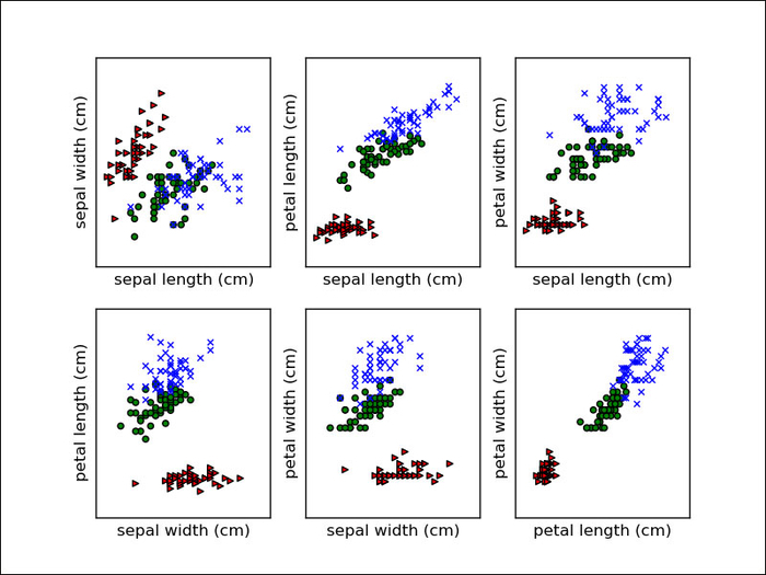
We are using Matplotlib; it is the most well-known plotting package for Python. We present the code to generate the top-left plot. The code for the other plots is similar to the following code:
from matplotlib import pyplot as plt
from sklearn.datasets import load_iris
import numpy as np

# We load the data with load_iris from sklearn
data = load_iris()
features = data['data']
feature_names = data['feature_names']
target = data['target']

for t,marker,c in zip(xrange(3),">ox","rgb"):
    # We plot each class on its own to get different colored markers
    plt.scatter(features[target == t,0],
                features[target == t,1],
                marker=marker,
c=c)If the goal is to separate the three types of flower, we can immediately make a few suggestions. For example, the petal length seems to be able to separate Iris Setosa from the other two flower species on its own. We can write a little bit of code to discover where the cutoff is as follows:
plength = features[:, 2]
# use numpy operations to get setosa features
is_setosa = (labels == 'setosa')
# This is the important step:
max_setosa =plength[is_setosa].max()
min_non_setosa = plength[~is_setosa].min()
print('Maximum of setosa: {0}.'.format(max_setosa))
print('Minimum of others: {0}.'.format(min_non_setosa))
This prints 1.9 and 3.0. Therefore, we can build a simple model: if the petal length is smaller than two, this is an Iris Setosa flower; otherwise, it is either Iris Virginica or Iris Versicolor.
if features[:,2] < 2: print 'Iris Setosa'
else: print 'Iris Virginica or Iris Versicolour'
This is our first model, and it works very well in that it separates the Iris Setosa flowers from the other two species without making any mistakes.
What we had here was a simple structure; a simple threshold on one of the dimensions. Then we searched for the best dimension threshold. We performed this visually and with some calculation; machine learning happens when we write code to perform this for us.
The example where we distinguished Iris Setosa from the other two species was very easy. However, we cannot immediately see what the best threshold is for distinguishing Iris Virginica from Iris Versicolor. We can even see that we will never achieve perfect separation. We can, however, try to do it the best possible way. For this, we will perform a little computation.
We first select only the non-Setosa features and labels:
features = features[~is_setosa]
labels = labels[~is_setosa]
virginica = (labels == 'virginica')
Here we are heavily using NumPy operations on the arrays. is_setosa is a Boolean array, and we use it to select a subset of the other two arrays, features and labels. Finally, we build a new Boolean array, virginica, using an equality comparison on labels.
Now, we run a loop over all possible features and thresholds to see which one results in better accuracy. Accuracy is simply the fraction of examples that the model classifies correctly:
best_acc = -1.0
for fi in xrange(features.shape[1]):
  # We are going to generate all possible threshold for this feature
  thresh = features[:,fi].copy()
  thresh.sort()
  # Now test all thresholds:
  for t in thresh:
    pred = (features[:,fi] > t)
    acc = (pred == virginica).mean()
    if acc > best_acc:
      best_acc = acc
      best_fi = fi
      best_t = t
The last few lines select the best model. First we compare the predictions, pred, with the actual labels, virginica. The little trick of computing the mean of the comparisons gives us the fraction of correct results, the accuracy. At the end of the for loop, all possible thresholds for all possible features have been tested, and the best_fi and best_t variables hold our model. To apply it to a new example, we perform the following:
if example[best_fi] > t: print 'virginica'
else: print 'versicolor'
What does this model look like? If we run it on the whole data, the best model that we get is split on the petal length. We can visualize the decision boundary. In the following screenshot, we see two regions: one is white and the other is shaded in grey. Anything that falls in the white region will be called Iris Virginica and anything that falls on the shaded side will be classified as Iris Versicolor:
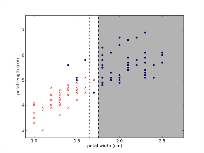
In a threshold model, the decision boundary will always be a line that is parallel to one of the axes. The plot in the preceding screenshot shows the decision boundary and the two regions where the points are classified as either white or grey. It also shows (as a dashed line) an alternative threshold that will achieve exactly the same accuracy. Our method chose the first threshold, but that was an arbitrary choice.
The model discussed in the preceding section is a simple model; it achieves 94 percent accuracy on its training data. However, this evaluation may be overly optimistic. We used the data to define what the threshold would be, and then we used the same data to evaluate the model. Of course, the model will perform better than anything else we have tried on this dataset. The logic is circular.
What we really want to do is estimate the ability of the model to generalize to new instances. We should measure its performance in instances that the algorithm has not seen at training. Therefore, we are going to do a more rigorous evaluation and use held-out data. For this, we are going to break up the data into two blocks: on one block, we'll train the model, and on the other—the one we held out of training—we'll test it. The output is as follows:
Training error was 96.0%.
Testing error was 90.0% (N = 50).
The result of the testing data is lower than that of the training error. This may surprise an inexperienced machine learner, but it is expected and typical. To see why, look back at the plot that showed the decision boundary. See if some of the examples close to the boundary were not there or if one of the ones in between the two lines was missing. It is easy to imagine that the boundary would then move a little bit to the right or to the left so as to put them on the "wrong" side of the border.
These concepts will become more and more important as the models become more complex. In this example, the difference between the two errors is not very large. When using a complex model, it is possible to get 100 percent accuracy in training and do no better than random guessing on testing!
One possible problem with what we did previously, which was to hold off data from training, is that we only used part of the data (in this case, we used half of it) for training. On the other hand, if we use too little data for testing, the error estimation is performed on a very small number of examples. Ideally, we would like to use all of the data for training and all of the data for testing as well.
We can achieve something quite similar by cross-validation. One extreme (but sometimes useful) form of cross-validation is leave-one-out. We will take an example out of the training data, learn a model without this example, and then see if the model classifies this example correctly:
error = 0.0
for ei in range(len(features)):
    # select all but the one at position 'ei':
        training = np.ones(len(features), bool)
        training[ei] = False
        testing = ~training
        model = learn_model(features[training], virginica[training])
        predictions = apply_model(features[testing],virginica[testing], model)
      error += np.sum(predictions != virginica[testing])
At the end of this loop, we will have tested a series of models on all the examples. However, there is no circularity problem because each example was tested on a model that was built without taking the model into account. Therefore, the overall estimate is a reliable estimate of how well the models would generalize.
The major problem with leave-one-out cross-validation is that we are now being forced to perform 100 times more work. In fact, we must learn a whole new model for each and every example, and this will grow as our dataset grows.
We can get most of the benefits of leave-one-out at a fraction of the cost by using x-fold cross-validation; here, "x" stands for a small number, say, five. In order to perform five-fold cross-validation, we break up the data in five groups, that is, five folds.
Then we learn five models, leaving one fold out of each. The resulting code will be similar to the code given earlier in this section, but here we leave 20 percent of the data out instead of just one element. We test each of these models on the left out fold and average the results:
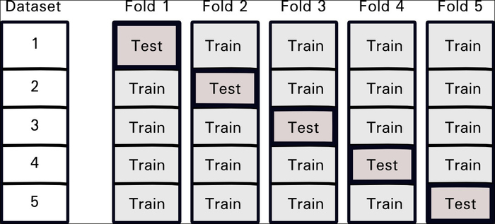
The preceding figure illustrates this process for five blocks; the dataset is split into five pieces. Then for each fold, you hold out one of the blocks for testing and train on the other four. You can use any number of folds you wish. Five or ten fold is typical; it corresponds to training with 80 or 90 percent of your data and should already be close to what you would get from using all the data. In an extreme case, if you have as many folds as datapoints, you can simply perform leave-one-out cross-validation.
When generating the folds, you need to be careful to keep them balanced. For example, if all of the examples in one fold come from the same class, the results will not be representative. We will not go into the details of how to do this because the machine learning packages will handle it for you.
We have now generated several models instead of just one. So, what final model do we return and use for the new data? The simplest solution is now to use a single overall model on all your training data. The cross-validation loop gives you an estimate of how well this model should generalize.
Although it was not properly recognized when machine learning was starting out, nowadays it is seen as a very bad sign to even discuss the training error of a classification system. This is because the results can be very misleading. We always want to measure and compare either the error on a held-out dataset or the error estimated using a cross-validation schedule.