A relatively recent development in the computer vision world has been the development of local-feature-based methods. Local features are computed on a small region of the image, unlike the previous features we considered, which had been computed on the whole image. Mahotas supports computing a type of these features; Speeded Up Robust Features, also known as SURF (there are several others, the most well-known being the original proposal of Scale-Invariant Feature Transform (SIFT)). These local features are designed to be robust against rotational or illumination changes (that is, they only change their value slightly when illumination changes).

When using these features, we have to decide where to compute them. There are three possibilities that are commonly used:

All of these are valid and will, under the right circumstances, give good results. Mahotas supports all three. Using interest point detection works best if you have a reason to expect that your interest point will correspond to areas of importance in the image. This depends, naturally, on what your image collection consists of. Typically, this is found to work better in man-made images rather than natural scenes. Man-made scenes have stronger angles, edges, or regions of high contrast, which are the typical regions marked as interesting by these automated detectors.

Since we are using photographs of mostly natural scenes, we are going to use the interest point method. Computing them with mahotas is easy; import the right submodule and call the surf.surf function:

from mahotas.features import surf
descriptors = surf.surf(image, descriptors_only=True)

The descriptors_only=True flag means that we are only interested in the descriptors themselves, and not in their pixel location, size, and other method information. Alternatively, we could have used the dense sampling method, using the surf.dense function:

from mahotas.features import surf
descriptors = surf.dense(image, spacing=16)

This returns the value of the descriptors computed on points that are at a distance of 16 pixels from each other. Since the position of the points is fixed, the meta-information on the interest points is not very interesting and is not returned by default. In either case, the result (descriptors) is an n-times-64 array, where n is the number of points sampled. The number of points depends on the size of your images, their content, and the parameters you pass to the functions. We used defaults previously, and this way we obtain a few hundred descriptors per image.

We cannot directly feed these descriptors to a support vector machine, logistic regressor, or similar classification system. In order to use the descriptors from the images, there are several solutions. We could just average them, but the results of doing so are not very good as they throw away all location-specific information. In that case, we would have just another global feature set based on edge measurements.

The solution we will use here is the bag-of-words model, which is a very recent idea. It was published in this form first in 2004. This is one of those "obvious in hindsight" ideas: it is very simple and works very well.

It may seem strange to say "words" when dealing with images. It may be easier to understand if you think that you have not written words, which are easy to distinguish from each other, but orally spoken audio. Now, each time a word is spoken, it will sound slightly different, so its waveform will not be identical to the other times it was spoken. However, by using clustering on these waveforms, we can hope to recover most of the structure so that all the instances of a given word are in the same cluster. Even if the process is not perfect (and it will not be), we can still talk of grouping the waveforms into words.

This is the same thing we do with visual words: we group together similar-looking regions from all images and call these visual words. Grouping is a form of clustering that we first encountered in Chapter 3, Clustering – Finding Related Posts.

We are going to start by computing the features:

alldescriptors = []
for im in images:
  im = mh.imread(im, as_grey=True)
  im = im.astype(np.uint8)
  alldescriptors.append(surf.surf(im, descriptors_only))

This results in over 100,000 local descriptors. Now, we use k-means clustering to obtain the centroids. We could use all the descriptors, but we are going to use a smaller sample for extra speed:

concatenated = np.concatenate(alldescriptors) # get all descriptors into a single array
concatenated = concatenated[::32] # use only every 32nd vector
from sklearn.cluster import Kmeans
k = 256
km = KMeans(k)
km.fit(concatenated)

After this is done (which will take a while), we have km containing information about the centroids. We now go back to the descriptors and build feature vectors:

features = []
for d in alldescriptors:
  c = km.predict(d)
  features.append(
      np.array([np.sum(c == ci) for ci in range(k)])
  )
features = np.array(features)

The end result of this loop is that features[fi] is a histogram corresponding to the image at position fi (the same could have been computed faster with the np.histogram function, but getting the arguments just right is a little tricky, and the rest of the code is, in any case, much slower than this simple step).

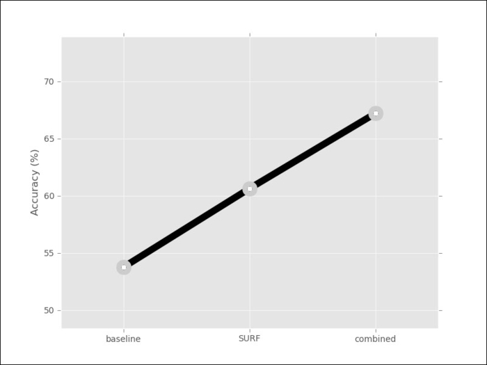
The result is that each image is now represented by a single array of features of the same size (the number of clusters; in our case 256). Therefore, we can use our standard classification methods. Using logistic regression again, we now get 62 percent, a 7 percent improvement. We can combine all of the features together and we obtain 67 percent, more than 12 percent over what was obtained with texture-based methods: