We will now turn to an example which comes from a study performed at Carnegie Mellon University by Prof. Noah Smith's research group. The study was based on mining the so-called "10-K reports" that companies file with the Securities and Exchange Commission (SEC) in the United States. This filing is mandated by the law for all publicly-traded companies. The goal is to predict, based on this piece of public information, what the future volatility of the company's stock will be. In the training data, we are actually using historical data for which we already know what happened.

There are 16,087 examples available. The features correspond to different words, 150,360 in total, which have already been preprocessed for us. Thus, we have many more features than examples.

The dataset is available in SVMLight format from multiple sources, including the book's companion website. This is a format which scikit-learn can read. SVMLight is, as the name says, a support vector machine implementation, which is also available through scikit-learn; right now, we are only interested in the file format.

from sklearn.datasets import load_svmlight_file
data,target = load_svmlight_file('E2006.train')

In the preceding code, data is a sparse matrix (that is, most of its entries are zeros and, therefore, only the non-zero entries are saved in memory), while target is a simple one-dimensional vector. We can start by looking at some attributes of target:

print('Min target value: {}'.format(target.min()))
print('Max target value: {}'.format(target.max()))
print('Mean target value: {}'.format(target.mean()))
print('Std. dev. target: {}'.format(target.std()))

This prints out the following values:

Min target value: -7.89957807347
Max target value: -0.51940952694
Mean target value: -3.51405313669
Std. dev. target: 0.632278353911

So, we can see that the data lies between -7.9 and -0.5. Now that we have an estimate data, we can check what happens when we use OLS to predict. Note that we can use exactly the same classes and methods as before:

from sklearn.linear_model import LinearRegression
lr = LinearRegression(fit_intercept=True)
lr.fit(data,target)
p = np.array(map(lr.predict, data))
p = p.ravel() # p is a (1,16087) array, we want to flatten it
e = p-target # e is 'error': difference of prediction and reality
total_sq_error = np.sum(e*e)
rmse_train = np.sqrt(total_sq_error/len(p))
print(rmse_train)

The error is not exactly zero because of the rounding error, but it is very close: 0.0025 (much smaller than the standard deviation of the target, which is the natural comparison value).

When we use cross-validation (the code is very similar to what we used before in the Boston example), we get something very different: 0.78. Remember that the standard deviation of the data is only 0.6. This means that if we always "predict" the mean value of -3.5, we have a root mean square error of 0.6! So, with OLS, in training, the error is insignificant. When generalizing, it is very large and the prediction is actually harmful: we would have done better (in terms of root mean square error) by simply predicting the mean value every time!

One solution, naturally, is to use regularization to counteract the overfitting. We can try the same cross-validation loop with an elastic net learner, having set the penalty parameter to 1. Now, we get 0.4 RMSE, which is better than just "predicting the mean". In a real-life problem, it is hard to know when we have done all we can as perfect prediction is almost always impossible.

In the preceding example, we set the penalty parameter to 1. We could just as well have set it to 2 (or half, or 200, or 20 million). Naturally, the results vary each time. If we pick an overly large value, we get underfitting. In extreme case, the learning system will just return every coefficient equal to zero. If we pick a value that is too small, we overfit and are very close to OLS, which generalizes poorly.

How do we choose a good value? This is a general problem in machine learning: setting parameters for our learning methods. A generic solution is to use cross-validation. We pick a set of possible values, and then use cross-validation to choose which one is best. This performs more computation (ten times more if we use 10 folds), but is always applicable and unbiased.

We must be careful, though. In order to obtain an estimate of generalization, we have to use two levels of cross-validation: one level is to estimate the generalization, while the second level is to get good parameters. That is, we split the data in, for example, 10 folds. We start by holding out the first fold and will learn on the other nine. Now, we split these again into 10 folds in order to choose the parameters. Once we have set our parameters, we test on the first fold. Now, we repeat this nine other times.

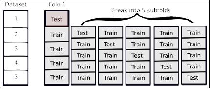
The preceding figure shows how you break up a single training fold into subfolds. We would need to repeat it for all the other folds. In this case, we are looking at five outer folds and five inner folds, but there is no reason to use the same number of outer and inner folds; you can use any numbers you want as long as you keep them separate.

This leads to a lot of computation, but it is necessary in order to do things correctly. The problem is that if you use a piece of data to make any decisions about your model (including which parameters to set), you have contaminated it and you can no longer use it to test the generalization ability of your model. This is a subtle point and it may not be immediately obvious. In fact, it is still the case that many users of machine learning get this wrong and overestimate how well their systems are doing because they do not perform cross-validation correctly!

Fortunately, scikit-learn makes it very easy to do the right thing: it has classes named LassoCV, RidgeCV, and ElasticNetCV, all of which encapsulate a cross-validation check for the inner parameter. The code is 100 percent like the previous one, except that we do not need to specify any value for alpha

from sklearn.linear_model import ElasticNetCV
met = ElasticNetCV(fit_intercept=True)
kf = KFold(len(target), n_folds=10)
for train,test in kf:
    met.fit(data[train],target[train])
    p = map(met.predict, data[test])
    p = np.array(p).ravel()
    e = p-target[test]
    err += np.dot(e,e)
rmse_10cv = np.sqrt(err/len(target))

This results in a lot of computation, so you may want to get some coffee while you are waiting (depending on how fast your computer is).

If you have used any commercial online system in the last 10 years, you have probably seen these recommendations. Some are like Amazon's "costumers who bought X also bought Y." These will be dealt with in the next chapter under the topic of basket analysis. Others are based on predicting the rating of a product, such as a movie.

This last problem was made famous with the Netflix Challenge; a million-dollar machine learning public challenge by Netflix. Netflix (well-known in the U.S. and U.K., but not available elsewhere) is a movie rental company. Traditionally, you would receive DVDs in the mail; more recently, the business has focused on online streaming of videos. From the start, one of the distinguishing features of the service was that it gave every user the option of rating films they had seen, using these ratings to then recommend other films. In this mode, you not only have the information about which films the user saw, but also their impression of them (including negative impressions).

In 2006, Netflix made available a large number of customer ratings of films in its database and the goal was to improve on their in-house algorithm for ratings prediction. Whoever was able to beat it by 10 percent or more would win 1 million dollars. In 2009, an international team named BellKor's Pragmatic Chaos was able to beat that mark and take the prize. They did so just 20 minutes before another team, The Ensemble, passed the 10 percent mark as well! An exciting photo-finish for a competition that lasted several years.

Unfortunately, for legal reasons, this dataset is no longer available (although the data was anonymous, there were concerns that it might be possible to discover who the clients were and reveal the private details of movie rentals). However, we can use an academic dataset with similar characteristics. This data comes from GroupLens, a research laboratory at the University of Minnesota.

We can formulate this as a regression problem and apply the methods that we learned in this chapter. It is not a good fit for a classification approach. We could certainly attempt to learn the five class classifiers, one class for each possible grade. There are two problems with this approach:

These two factors together mean that classification is not a good fit to the problem. The regression framework is more meaningful.

We have two choices: we can build movie-specific or user-specific models. In our case, we are going to first build user-specific models. This means that, for each user, we take the movies, it has rated as our target variable. The inputs are the ratings of other old users. This will give a high value to users who are similar to our user (or a negative value to users who like more or less the same movies that our user dislikes).

The system is just an application of what we have developed so far. You will find a copy of the dataset and code to load it into Python on the book's companion website. There you will also find pointers to more information, including the original MovieLens website.

The loading of the dataset is just basic Python, so let us jump ahead to the learning. We have a sparse matrix, where there are entries from 1 to 5 whenever we have a rating (most of the entries are zero to denote that this user has not rated these movies). This time, as a regression method, for variety, we are going to be using the LassoCV class:

from sklearn.linear_model import LassoCV
reg = LassoCV(fit_intercept=True, alphas=[.125,.25,.5,1.,2.,4.])

By passing the constructor an explicit set of alphas, we can constrain the values that the inner cross-validation will use. You may note that the values are multiples of two, starting with 1/8 up to 4. We will now write a function which learns a model for the user i:

# isolate this user
u = reviews[i]

We are only interested in the movies that the user u rated, so we must build up the index of those. There are a few NumPy tricks in here: u.toarray() to convert from a sparse matrix to a regular array. Then, we ravel() that array to convert from a row array (that is, a two-dimensional array with a first dimension of 1) to a simple one-dimensional array. We compare it with zero and ask where this comparison is true. The result, ps, is an array of indices; those indices correspond to movies that the user has rated:

u = u.array().ravel()
ps, = np.where(u > 0)

# Build an array with indices [0...N] except i
us = np.delete(np.arange(reviews.shape[0]), i)

x = reviews[us][:,ps].T

Finally, we select only the movies that the user has rated:

y = u[ps]

Cross-validation is set up as before. Because we have many users, we are going to only use four folds (more would take a long time and we have enough training data with just 80 percent of the data):

err = 0
kf = KFold(len(y), n_folds=4)
for train,test in kf:
      # Now we perform a per-movie normalization
      # this is explained below
      xc,x1 = movie_norm(x[train])
    reg.fit(xc, y[train]-x1)
    # We need to perform the same normalization while testing
    xc,x1 = movie_norm(x[test])
    p = np.array(map(reg.predict, xc)).ravel()
    e = (p+x1)-y[test]
    err += np.sum(e*e)

We did not explain the movie_norm function. This function performs per-movie normalization: some movies are just generally better and get higher average marks:

def movie_norm(x):
    xc = x.copy().toarray()

We cannot use xc.mean(1) because we do not want to have the zeros counting for the mean. We only want the mean of the ratings that were actually given:

    x1 = np.array([xi[xi > 0].mean() for xi in xc])

In certain cases, there were no ratings and we got a NaN value, so we replace it with zeros using np.nan_to_num, which does exactly this task:

    x1 = np.nan_to_num(x1)

Now we normalize the input by removing the mean value from the non-zero entries:

    for i in xrange(xc.shape[0]):
        xc[i] -= (xc[i] > 0) * x1[i]

Implicitly, this also makes the movies that the user did not rate have a value of zero, which is average. Finally, we return the normalized array and the means:

    return x,x1

You might have noticed that we converted to a regular (dense) array. This has the added advantage that it makes the optimization much faster: while scikit-learn works well with the sparse values, the dense arrays are much faster (if you can fit them in memory; when you cannot, you are forced to use sparse arrays).

When compared with simply guessing the average value for that user, this approach is 80 percent better. The results are not spectacular, but it is a start. On one hand, this is a very hard problem and we cannot expect to be right with every prediction: we perform better when the users have given us more reviews. On the other hand, regression is a blunt tool for this job. Note how we learned a completely separate model for each user. In the next chapter, we will look at other methods that go beyond regression for approaching this problem. In those models, we integrate the information from all users and all movies in a more intelligent manner.