As we have seen when we looked at our tweet data, the tweets are not just positive or negative. The majority of tweets actually do not contain any sentiment, but are neutral or irrelevant, containing, for instance, raw information (New book: Building Machine Learning ... http://link). This leads to four classes. To avoid complicating the task too much, let us for now only focus on the positive and negative tweets:

>>> pos_neg_idx=np.logical_or(Y=="positive", Y=="negative")
>>> X = X[pos_neg_idx]
>>> Y = Y[pos_neg_idx]
>>> Y = Y=="positive"

Now, we have in X the raw tweet texts and in Y the binary classification; we assign 0 for negative and 1 for positive tweets.

As we have learned in the chapters before, we can construct TfidfVectorizer to convert the raw tweet text into the TF-IDF feature values, which we then use together with the labels to train our first classifier. For convenience, we will use the Pipeline class, which allows us to join the vectorizer and the classifier together and provides the same interface:

from sklearn.feature_extraction.text import TfidfVectorizer
from sklearn.naive_bayes import MultinomialNB
from sklearn.pipeline import Pipeline

def create_ngram_model():
    tfidf_ngrams = TfidfVectorizer(ngram_range=(1, 3),analyzer="word", binary=False)
    clf = MultinomialNB()
    pipeline = Pipeline([('vect', tfidf_ngrams), ('clf', clf)])
    return pipeline

The Pipeline instance returned by create_ngram_model() can now be used for fit() and predict() as if we had a normal classifier.

Since we do not have that much data, we should do cross-validation. This time, however, we will not use KFold, which partitions the data in consecutive folds, but instead we use ShuffleSplit. This shuffles the data for us, but does not prevent the same data instance to be in multiple folds. For each fold, then, we keep track of the area under the Precision-Recall curve and the accuracy.

To keep our experimentation agile, let us wrap everything together in a train_model() function, which takes a function as a parameter that creates the classifier:

from sklearn.metrics import precision_recall_curve, auc
from sklearn.cross_validation import ShuffleSplit

def train_model(clf_factory, X, Y):
     # setting random_state to get deterministic behavior
    cv = ShuffleSplit(n=len(X), n_iter=10, test_size=0.3,indices=True, random_state=0)

    scores = []
    pr_scores = []

    for train, test in cv:
        X_train, y_train = X[train], Y[train]
        X_test, y_test = X[test], Y[test]

        clf = clf_factory()
        clf.fit(X_train, y_train)

        train_score = clf.score(X_train, y_train)
        test_score = clf.score(X_test, y_test)

        scores.append(test_score)
        proba = clf.predict_proba(X_test)

        precision, recall, pr_thresholds = precision_recall_curve(y_test, proba[:,1])

        pr_scores.append(auc(recall, precision))

    summary = (np.mean(scores), np.std(scores),
               np.mean(pr_scores), np.std(pr_scores))
    print "%.3f	%.3f	%.3f	%.3f"%summary

>>> X, Y = load_sanders_data()
>>> pos_neg_idx=np.logical_or(Y=="positive", Y=="negative")
>>> X = X[pos_neg_idx]
>>> Y = Y[pos_neg_idx]
>>> Y = Y=="positive"
>>> train_model(create_ngram_model)
0.805    0.024    0.878    0.016

With our first try of using Naive Bayes on vectorized TF-IDF trigram features, we get an accuracy of 80.5 percent and a P/R AUC of 87.8 percent. Looking at the P/R chart shown in the following screenshot, it shows a much more encouraging behavior than the plots we saw in the previous chapter:

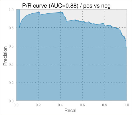
For the first time, the results are quite encouraging. They get even more impressive when we realize that 100 percent accuracy is probably never achievable in a sentiment classification task. For some tweets, even humans often do not really agree on the same classification label.

But again, we simplified our task a bit, since we used only positive or negative tweets. That means we assumed a perfect classifier that classified upfront whether the tweet contains a sentiment and forwarded that to our Naive Bayes classifier.

So, how well do we perform if we also classify whether a tweet contains any sentiment at all? To find that out, let us first write a convenience function that returns a modified class array that provides a list of sentiments that we would like to interpret as positive

def tweak_labels(Y, pos_sent_list):
    pos = Y==pos_sent_list[0]
    for sent_label in pos_sent_list[1:]:
pos |= Y==sent_label

    Y = np.zeros(Y.shape[0])
    Y[pos] = 1
    Y = Y.astype(int)

    return Y

Note that we are talking about two different positives now. The sentiment of a tweet can be positive, which is to be distinguished from the class of the training data. If, for example, we want to find out how good we can separate the tweets having sentiment from neutral ones, we could do this as follows:

>>> Y = tweak_labels(Y, ["positive", "negative"])

In Y we now have a 1 (positive class) for all tweets that are either positive or negative and a 0 (negative class) for neutral and irrelevant ones.

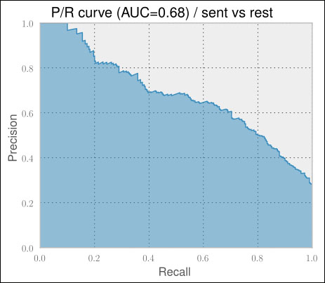
>>> train_model(create_ngram_model, X, Y, plot=True)
0.767    0.014    0.670    0.022

As expected, the P/R AUC drops considerably, being only 67 percent now. The accuracy is still high, but that is only due to the fact that we have a highly imbalanced dataset. Out of 3,642 total tweets, only 1,017 are either positive or negative, which is about 28 percent. This means that if we created a classifier that always classified a tweet as not containing any sentiments, we would already have an accuracy of 72 percent. This is another example of why you should always look at precision and recall if the training and test data is unbalanced.

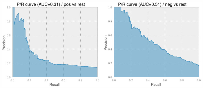
So, how would the Naive Bayes classifier perform on classifying positive tweets versus the rest and negative tweets versus the rest? One word: bad.

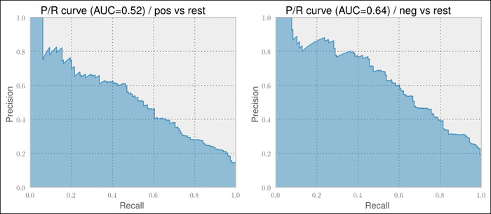
== Pos vs. rest ==
0.866    0.010    0.327    0.017    
== Neg vs. rest ==
0.861    0.010    0.560    0.020    

Pretty unusable if you ask me. Looking at the P/R curves shown in the following screenshots, we also find no usable precision/recall tradeoff as we were able to do in the previous chapter.

Certainly, we have not explored the current setup enough and should investigate more. There are roughly two areas where we could play with the knobs: TfidfVectorizer and MultinomialNB. As we have no real intuition as to which area we should explore, let us try to distribute the parameters' values:

A simple approach could be to train a classifier for all those reasonable exploration values while keeping the other parameters constant and checking the classifier's results. As we do not know whether those parameters affect each other, doing it right would require that we train a classifier for every possible combination of all parameter values. Obviously, this is too tedious for us to do.

Because this kind of parameter exploration occurs frequently in machine learning tasks, scikit-learn has a dedicated class for it called GridSearchCV. It takes an estimator (an instance with a classifier-like interface), which would be the pipeline instance in our case, and a dictionary of parameters with their potential values.

GridSearchCV expects the dictionary's keys to obey a certain format so that it is able to set the parameters of the correct estimator. The format is as follows:

<estimator>__<subestimator>__...__<param_name>

Now, if we want to specify the desired values to explore for the min_df parameter of TfidfVectorizer (named vect in the Pipeline description), we would have to say:

Param_grid={"vect__ngram_range"=[(1, 1), (1, 2), (1, 3)]}

This would tell GridSearchCV to try out unigrams, bigrams, and trigrams as parameter values for the ngram_range parameter of TfidfVectorizer.

Then it trains the estimator with all possible parameter/value combinations. Finally, it provides the best estimator in the form of the member variable best_estimator_.

As we want to compare the returned best classifier with our current best one, we need to evaluate it the same way. Therefore, we can pass the ShuffleSplit instance using the CV parameter (this is the reason CV is present in GridSearchCV).

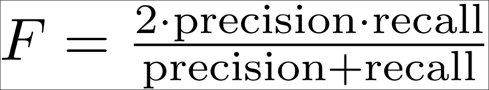
The only missing thing is to define how GridSearchCV should determine the best estimator. This can be done by providing the desired score function to (surprise!) the score_func parameter. We could either write one ourselves or pick one from the sklearn.metrics package. We should certainly not take metric.accuracy because of our class imbalance (we have a lot less tweets containing sentiment than neutral ones). Instead, we want to have good precision and recall on both the classes: the tweets with sentiment and the tweets without positive or negative opinions. One metric that combines both precision and recall is the F-measure metric, which is implemented as metrics.f1_score:

Putting everything together, we get the following code:

from sklearn.grid_search import GridSearchCV
from sklearn.metrics import f1_score

def grid_search_model(clf_factory, X, Y):
    cv = ShuffleSplit(
        n=len(X), n_iter=10, test_size=0.3, indices=True, random_state=0)

    param_grid = dict(vect__ngram_range=[(1, 1), (1, 2), (1, 3)],
                      vect__min_df=[1, 2],
                      vect__stop_words=[None, "english"],
                      vect__smooth_idf=[False, True],
                      vect__use_idf=[False, True],
                      vect__sublinear_tf=[False, True],
                      vect__binary=[False, True],
                      clf__alpha=[0, 0.01, 0.05, 0.1, 0.5, 1],
                      )

    grid_search = GridSearchCV(clf_factory(),
                               param_grid=param_grid,
                               cv=cv,
                               score_func=f1_score,
                               verbose=10)
    grid_search.fit(X, Y) 
 
    return grid_search.best_estimator_

We have to be patient when executing the following code:

clf = grid_search_model(create_ngram_model, X, Y)
print clf

This is because we have just requested a parameter sweep over the parameter combinations—each being trained on 10 folds:

... waiting some hours  ...
Pipeline(clf=MultinomialNB(
             alpha=0.01, class_weight=None, 
          fit_prior=True),
         clf__alpha=0.01, 
         clf__class_weight=None, 
         clf__fit_prior=True,
         vect=TfidfVectorizer(
              analyzer=word, binary=False,
                 charset=utf-8, charset_error=strict, 
              dtype=<type 'long'>, input=content,
              lowercase=True, max_df=1.0, 
              max_features=None, max_n=None,
              min_df=1, min_n=None, ngram_range=(1, 2),
              norm=l2, preprocessor=None, smooth_idf=False, 
              stop_words=None,strip_accents=None, 
              sublinear_tf=True, token_pattern=(?u)ww+,
              token_processor=None, tokenizer=None, 
              use_idf=False, vocabulary=None),
         vect__analyzer=word, vect__binary=False, 
         vect__charset=utf-8,
         vect__charset_error=strict, 
         vect__dtype=<type 'long'>,
         vect__input=content, vect__lowercase=True, 
         vect__max_df=1.0, vect__max_features=None, 
         vect__max_n=None, vect__min_df=1,
         vect__min_n=None, vect__ngram_range=(1, 2), 
         vect__norm=l2, vect__preprocessor=None, 
         vect__smooth_idf=False, vect__stop_words=None, 
         vect__strip_accents=None, vect__sublinear_tf=True,
         vect__token_pattern=(?u)ww+,
         vect__token_processor=None, vect__tokenizer=None,
         vect__use_idf=False, vect__vocabulary=None)
0.795    0.007    0.702    0.028     

The best estimator indeed improves the P/R AUC by nearly 3.3 percent to 70.2 with the setting that was printed earlier.

The devastating results for positive tweets against the rest and negative tweets against the rest will improve if we configure the vectorizer and classifier with those parameters that we have just found out:

== Pos vs. rest ==
0.883    0.005    0.520    0.028    
== Neg vs. rest ==
0.888    0.009    0.631    0.031        

Indeed, the P/R curves look much better (note that the graphs are from the medium of the fold classifiers, thus have slightly diverging AUC values):

Nevertheless, we probably still wouldn't use those classifiers. Time for something completely different!