You have probably learned about regression already in high school mathematics class, this was probably called ordinary least squares (OLS) regression then. This centuries old technique is fast to run and can be effectively used for many real-world problems. In this chapter, we will start by reviewing OLS regression and showing you how it is available in both NumPy and scikit-learn.
In various modern problems, we run into limitations of the classical methods and start to benefit from more advanced methods, which we will see later in this chapter. This is particularly true when we have many features, including when we have more features than examples (which is something that ordinary least squares cannot handle correctly). These techniques are much more modern, with major developments happening in the last decade. They go by names such as lasso, ridge, or elastic nets. We will go into these in detail.
Finally, we will start looking at recommendations. This is an important area in many applications as it is a significant added-value to many applications. This is a topic that we will start exploring here and will see in more detail in the next chapter.
Let us start with a simple problem, predicting house prices in Boston.
We can use a publicly available dataset. We are given several demographic and geographical attributes, such as the crime rate or the pupil-teacher ratio, and the goal is to predict the median value of a house in a particular area. As usual, we have some training data, where the answer is known to us.
We start by using scikit-learn's methods to load the dataset. This is one of the built-in datasets that scikit-learn comes with, so it is very easy:
from sklearn.datasets import load_boston
boston = load_boston()
The boston object is a composite object with several attributes, in particular, boston.data and boston.target will be of interest to us.
We will start with a simple one-dimensional regression, trying to regress the price on a single attribute according to the average number of rooms per dwelling, which is stored at position 5 (you can consult boston.DESCR and boston.feature_names for detailed information on the data):
from matplotlib import pyplot as plt
plt.scatter(boston.data[:,5], boston.target, color='r')
The boston.target attribute contains the average house price (our target variable). We can use the standard least squares regression you probably first saw in high school. Our first attempt looks like this:
import numpy as np
We import NumPy, as this basic package is all we need. We will use functions from the np.linalg submodule, which performs basic linear algebra operations:
x = boston.data[:,5]
x = np.array([[v] for v in x])
This may seem strange, but we want x to be two dimensional: the first dimension is the different examples, while the second dimension is the attributes. In our case, we have a single attribute, the mean number of rooms per dwelling, so the second dimension is 1:
y = boston.target
slope,_,_,_ = np.linalg.lstsq(x,y)
Finally, we use least squares regression to obtain the slope of the regression. The np.linalg.lstsq function also returns some internal information on how well the regression fits the data, which we will ignore for the moment.
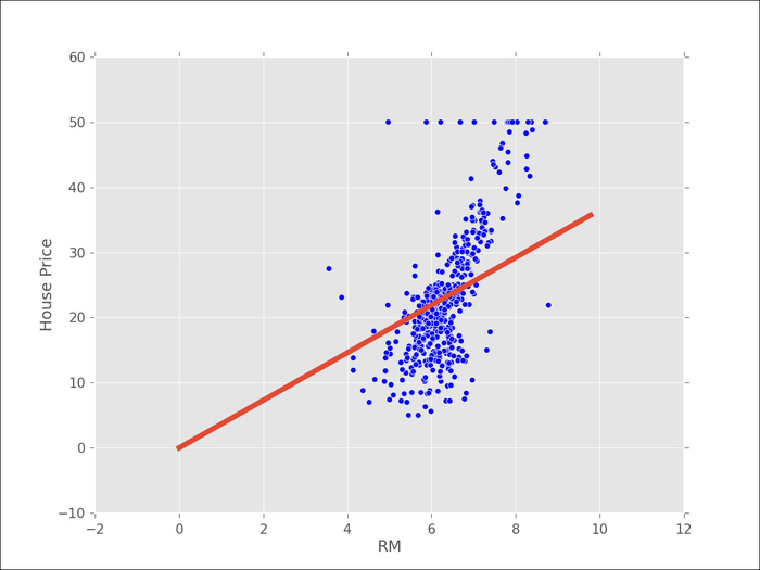
The preceding graph shows all the points (as dots) and our fit (the solid line). This does not look very good. In fact, using this one-dimensional model, we understand that House Price is a multiple of the RM variable (the number of rooms).
This would mean that, on average, a house with two rooms would be double the price of a single room and with three rooms would be triple the price. We know that these are false assumptions (and are not even approximately true).
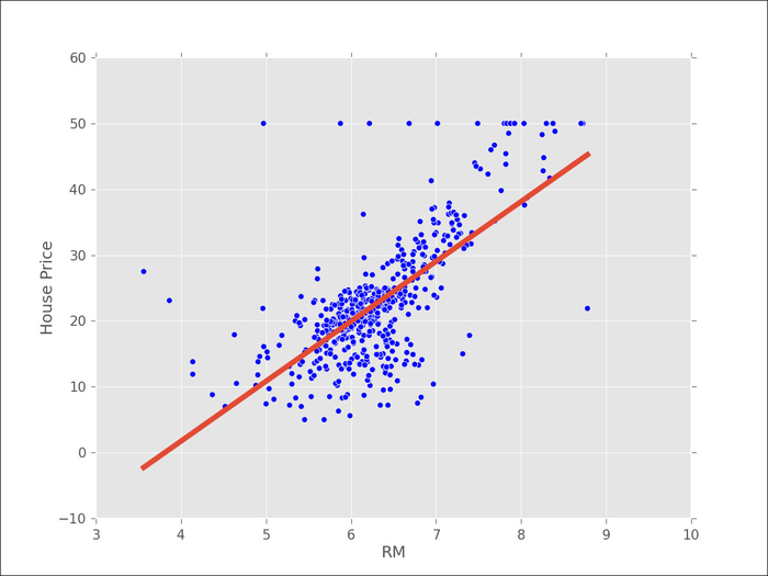
One common step is to add a bias term to the previous expression so that the price is a multiple of RM plus a bias. This bias is the base price for a zero-bedroom apartment. The trick to implement this is to add 1 to every element of x:
x = boston.data[:,5]
x = np.array([[v,1] for v in x]) # we now use [v,1] instead of [v]
    y = boston.target
(slope,bias),_,_,_ = np.linalg.lstsq(x,y)
In the following screenshot, we can see that visually it looks better (even though a few outliers may be having a disproportionate impact on the result):
Ideally, though, we would like to measure how good of a fit this is quantitatively. In order to do so, we can ask how close our prediction is. For this, we now look at one of those other returned values from the np.linalg.lstsq function, the second element:
(slope,bias),total_error,_,_ = np.linalg.lstsq(x,y)
rmse = np.sqrt(total_error[0]/len(x))
The np.linalg.lstsq function returns the total squared error. For each element, it checks the error (the difference between the line and the true value), squares it, and returns the sum of all these. It is more understandable to measure the average error, so we divide by the number of elements. Finally, we take the square root and print out the root mean squared error (RMSE). For the first unbiased regression, we get an error of 7.6, while adding the bias improves it to 6.6. This means that we can expect the price to be different from the real price by at the most 13 thousand dollars.
Tip
Root mean squared error and prediction
The root mean squared error corresponds approximately to an estimate of the standard deviation. Since most of the data is at the most two standard deviations from the mean, we can double our RMSE to obtain a rough confident interval. This is only completely valid if the errors are normally distributed, but it is roughly correct even if they are not.
So far, we have only used a single variable for prediction, the number of rooms per dwelling. We will now use all the data we have to fit a model using multidimensional regression. We now try to predict a single output (the average house price) based on multiple inputs.
The code looks very much like before:
x = boston.data
      # we still add a bias term, but now we must use np.concatenate, which
      # concatenates two arrays/lists because we
      # have several input variables in v
x = np.array([np.concatenate(v,[1]) for v in boston.data])
  y = boston.target
  s,total_error,_,_ = np.linalg.lstsq(x,y)
Now, the root mean squared error is only 4.7! This is better than what we had before, which indicates that the extra variables did help. Unfortunately, we can no longer easily display the results as we have a 14-dimensional regression.
If you remember when we first introduced classification, we stressed the importance of cross-validation for checking the quality of our predictions. In regression, this is not always done. In fact, we only discussed the training error model earlier. This is a mistake if you want to confidently infer the generalization ability. Since ordinary least squares is a very simple model, this is often not a very serious mistake (the amount of overfitting is slight). However, we should still test this empirically, which we will do now using scikit-learn. We will also use its linear regression classes as they will be easier to replace for more advanced methods later in the chapter:
from sklearn.linear_model import LinearRegression
The LinearRegression class implements OLS regression as follows:
lr = LinearRegression(fit_intercept=True)
We set the fit_intercept parameter to True in order to add a bias term. This is exactly what we had done before, but in a more convenient interface:
lr.fit(x,y)
p = map(lr.predict, x)
Learning and prediction are performed for classification as follows:
e = p-y
total_error = np.sum(e*e) # sum of squares
rmse_train = np.sqrt(total_error/len(p))
print('RMSE on training: {}'.format(rmse_train))
We have used a different procedure to compute the root mean square error on the training data. Of course, the result is the same as we had before: 4.6 (it is always good to have these sanity checks to make sure we are doing things correctly).
Now, we will use the KFold class to build a 10-fold cross-validation loop and test the generalization ability of linear regression:
from sklearn.cross_validation import Kfold
kf = KFold(len(x), n_folds=10)
err = 0
for train,test in kf:
    lr.fit(x[train],y[train])
    p = map(lr.predict, x[test])
    e = p-y[test]
    err += np.sum(e*e)
rmse_10cv = np.sqrt(err/len(x))
print('RMSE on 10-fold CV: {}'.format(rmse_10cv))
With cross-validation, we obtain a more conservative estimate (that is, the error is greater): 5.6. As in the case of classification, this is a better estimate of how well we could generalize to predict prices.
Ordinary least squares is fast at learning time and returns a simple model, which is fast at prediction time. For these reasons, it should often be the first model that you use in a regression problem. However, we are now going to see more advanced methods.