We will now look at another agricultural dataset; it is still small, but now too big to comfortably plot exhaustively as we did with Iris. This is a dataset of the measurements of wheat seeds. Seven features are present, as follows:

There are three classes that correspond to three wheat varieties: Canadian, Koma, and Rosa. As before, the goal is to be able to classify the species based on these morphological measurements.

Unlike the Iris dataset, which was collected in the 1930s, this is a very recent dataset, and its features were automatically computed from digital images.

This is how image pattern recognition can be implemented: you can take images in digital form, compute a few relevant features from them, and use a generic classification system. In a later chapter, we will work through the computer vision side of this problem and compute features in images. For the moment, we will work with the features that are given to us.

One interesting aspect of these features is that the compactness feature is not actually a new measurement, but a function of the previous two features, area and perimeter. It is often very useful to derive new combined features. This is a general area normally termed feature engineering; it is sometimes seen as less glamorous than algorithms, but it may matter more for performance (a simple algorithm on well-chosen features will perform better than a fancy algorithm on not-so-good features).

In this case, the original researchers computed the "compactness", which is a typical feature for shapes (also called "roundness"). This feature will have the same value for two kernels, one of which is twice as big as the other one, but with the same shape. However, it will have different values for kernels that are very round (when the feature is close to one) as compared to kernels that are elongated (when the feature is close to zero).

The goals of a good feature are to simultaneously vary with what matters and be invariant with what does not. For example, compactness does not vary with size but varies with the shape. In practice, it might be hard to achieve both objectives perfectly, but we want to approximate this ideal.

You will need to use background knowledge to intuit which will be good features. Fortunately, for many problem domains, there is already a vast literature of possible features and feature types that you can build upon. For images, all of the previously mentioned features are typical, and computer vision libraries will compute them for you. In text-based problems too, there are standard solutions that you can mix and match (we will also see this in a later chapter). Often though, you can use your knowledge of the specific problem to design a specific feature.

Even before you have data, you must decide which data is worthwhile to collect. Then, you need to hand all your features to the machine to evaluate and compute the best classifier.

A natural question is whether or not we can select good features automatically. This problem is known as feature selection. There are many methods that have been proposed for this problem, but in practice, very simple ideas work best. It does not make sense to use feature selection in these small problems, but if you had thousands of features, throwing out most of them might make the rest of the process much faster.

With this dataset, even if we just try to separate two classes using the previous method, we do not get very good results. Let me introduce , therefore, a new classifier: the nearest neighbor classifier.

If we consider that each example is represented by its features (in mathematical terms, as a point in N-dimensional space), we can compute the distance between examples. We can choose different ways of computing the distance, for example:

  def distance(p0, p1):
    'Computes squared euclidean distance'
    return np.sum( (p0-p1)**2)

Now when classifying, we adopt a simple rule: given a new example, we look at the dataset for the point that is closest to it (its nearest neighbor) and look at its label:

def nn_classify(training_set, training_labels, new_example):
  dists = np.array([distance(t, new_example)
      for t in training_set])
  nearest = dists.argmin()
  return training_labels[nearest]

In this case, our model involves saving all of the training data and labels and computing everything at classification time. A better implementation would be to actually index these at learning time to speed up classification, but this implementation is a complex algorithm.

Now, note that this model performs perfectly on its training data! For each point, its closest neighbor is itself, and so its label matches perfectly (unless two examples have exactly the same features but different labels, which can happen). Therefore, it is essential to test using a cross-validation protocol.

Using ten folds for cross-validation for this dataset with this algorithm, we obtain 88 percent accuracy. As we discussed in the earlier section, the cross-validation accuracy is lower than the training accuracy, but this is a more credible estimate of the performance of the model.

We will now examine the decision boundary. For this, we will be forced to simplify and look at only two dimensions (just so that we can plot it on paper).

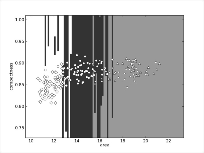
In the preceding screenshot, the Canadian examples are shown as diamonds, Kama seeds as circles, and Rosa seeds as triangles. Their respective areas are shown as white, black, and grey. You might be wondering why the regions are so horizontal, almost weirdly so. The problem is that the x axis (area) ranges from 10 to 22 while the y axis (compactness) ranges from 0.75 to 1.0. This means that a small change in x is actually much larger than a small change in y. So, when we compute the distance according to the preceding function, we are, for the most part, only taking the x axis into account.

If you have a physics background, you might have already noticed that we had been summing up lengths, areas, and dimensionless quantities, mixing up our units (which is something you never want to do in a physical system). We need to normalize all of the features to a common scale. There are many solutions to this problem; a simple one is to normalize to Z-scores. The Z-score of a value is how far away from the mean it is in terms of units of standard deviation. It comes down to this simple pair of operations:

# subtract the mean for each feature:
features -= features.mean(axis=0)
# divide each feature by its standard deviation
features /= features.std(axis=0)

Independent of what the original values were, after Z-scoring, a value of zero is the mean and positive values are above the mean and negative values are below it.

Now every feature is in the same unit (technically, every feature is now dimensionless; it has no units) and we can mix dimensions more confidently. In fact, if we now run our nearest neighbor classifier, we obtain 94 percent accuracy!

Look at the decision space again in two dimensions; it looks as shown in the following screenshot:

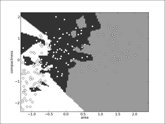
The boundaries are now much more complex and there is interaction between the two dimensions. In the full dataset, everything is happening in a seven-dimensional space that is very hard to visualize, but the same principle applies: where before a few dimensions were dominant, now they are all given the same importance.

The nearest neighbor classifier is simple, but sometimes good enough. We can generalize it to a k-nearest neighbor classifier by considering not just the closest point but the k closest points. All k neighbors vote to select the label. k is typically a small number, such as 5, but can be larger, particularly if the dataset is very large.