We will start with a small dataset that was collected especially for this book. It has three classes: buildings, natural scenes (landscapes), and pictures of texts. There are 30 images in each category, and they were all taken using a cell phone camera with minimal composition, so the images are similar to those that would be uploaded to a modern website. This dataset is available from the book's website. Later in the chapter, we will look at a harder dataset with more images and more categories.

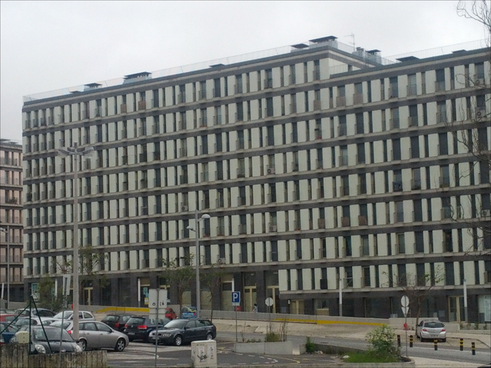
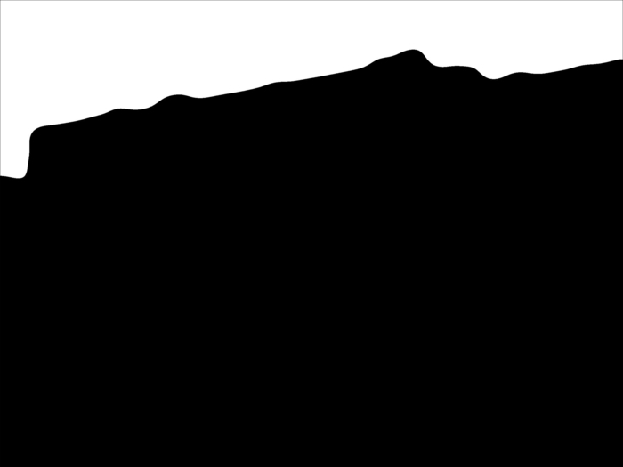
This screenshot of a building is one of the images in the dataset. We will use this screenshot as an example.

As you may be aware, image processing is a large field. Here we will only be looking at some very basic operations we can perform on our images. Some of the most basic operations can be performed using NumPy only, but otherwise we will use mahotas.

Thresholding

Thresholding is a very simple operation: we transform all pixel values above a certain threshold to 1 and all those below to 0 (or by using Booleans, transform it to True and False):

binarized = (image > threshold_value)

The value of the threshold width (threshold_value in the code) needs to be chosen. If the images are all very similar, we can pick one statically and use it for all images. Otherwise, we must compute a different threshold for each image based on its pixel values.

Mahotas implements a few methods for choosing a threshold value. One is called Otsu , after its inventor. The first necessary step is to convert the image to grayscale with rgb2gray.

Instead of rgb2gray, we can also have just the mean value of the red, green, and blue channels by calling image.mean(2). The result, however, will not be the same because rgb2gray uses different weights for the different colors to give a subjectively more pleasing result. Our eyes are not equally sensitive to the three basic colors.

image = mh.colors.rgb2gray(image, dtype=np.uint8)
plt.imshow(image) # Display the image

By default, matplotlib will display this single-channel image as a false color image, using red for high values and blue for low. For natural images, grayscale is more appropriate. You can select it with the following:

plt.gray()

Now the screenshot is shown in grayscale. Note that only the way in which the pixel values are interpreted and shown has changed and the screenshot is untouched. We can continue our processing by computing the threshold value.

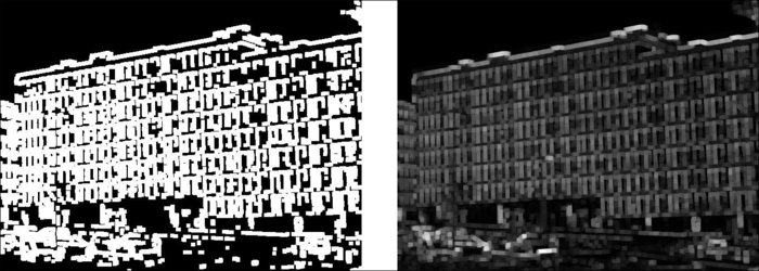
thresh = mh.thresholding.otsu(image)
print(thresh)
imshow(image > thresh)

When applied to the previous screenshot, this method finds the threshold 164 value, which separates the building and parked cars from the sky above.

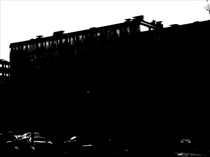
The result may be useful on its own (if you are measuring some properties of the thresholded image) or it can be useful for further processing. The result is a binary image that can be used to select a region of interest.

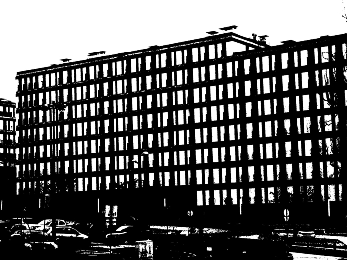
The result is still not very good. We can use operations on this screenshot to further refine it. For example, we can run the close operator to get rid of some of the noise in the upper corners.

otsubin =  (image <= thresh)
otsubin =  mh.close(otsubin, np.ones((15,15)))

In this case, we are closing the region that is below the threshold, so we reversed the threshold operator. We could, alternatively, have performed an open operation on the negative of the image.

otsubin =  (image > thresh)
otsubin =  mh.open(otsubin, np.ones((15,15)))

In either case, the operator takes a structuring element that defines the type of region we want to close. In our case, we used a 15x15 square.

This is still not perfect as there are a few bright objects in the parking lot that are not picked up. We will improve it a bit later in the chapter.

The Otsu threshold was able to identify the region of the sky as brighter than the building. An alternative thresholding method is the Ridley-Calvard method (also named after its inventors):

thresh = mh.thresholding.rc(image)
print(thresh)

This method returns a smaller threshold, 137.7, and tells apart the building details.

Whether this is better or worse depends on what you are trying to distinguish.

Gaussian blurring

Blurring your image may seem odd, but it often serves to reduce noise, which helps with further processing. With mahotas, it is just a function call:

image = mh.colors.rgb2gray(image)
im8 = mh.gaussian_filter(image,8)

Notice how we did not convert the gray screenshot to unsigned integers; we just made use of the floating point result as it is. The second argument to the gaussian_filter function is the size of the filter (the standard deviation of the filter). Larger values result in more blurring, as can be seen in the following screenshot (shown are filtering with sizes 8, 16, and 32):

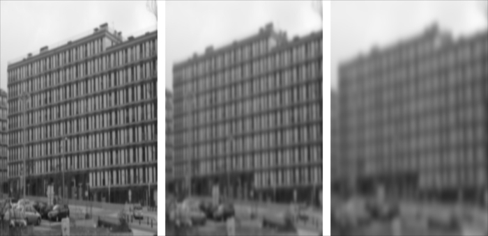
We can use the screenshot on the left and threshold it with Otsu (using the same code seen previously). Now the result is a perfect separation of the building region and the sky. While some of the details have been smoothed over, the bright regions in the parking lot have also been smoothed over. The result is an approximate outline of the sky without any artifacts. By blurring, we got rid of the detail that didn't matter to the broad picture. Have a look at the following screenshot:

Filtering for different effects

The use of image processing to achieve pleasing effects in images dates back to the beginning of digital images, but it has recently been the basis of a number of interesting applications, the most well-known of which is probably Instagram.

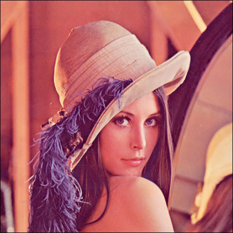
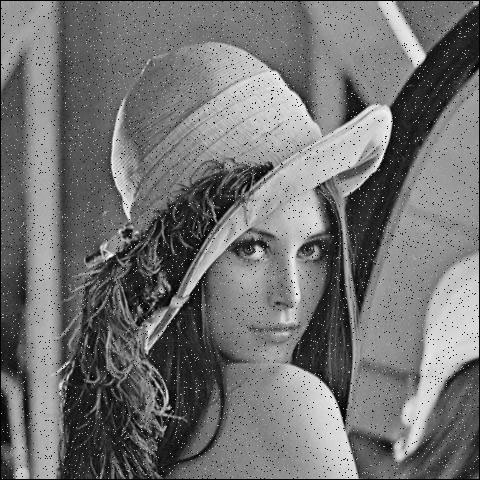
We are going to use a traditional image in image processing, the screenshot of the Lenna image, which is shown and can be downloaded from the book's website (or many other image-processing websites):

im = mh.imread('lenna.jpg', as_grey=True)

We can perform many further manipulations on this result if we want to. For example, we will now add a bit of salt and pepper noise to the image to simulate a few scanning artifacts. We generate random arrays of the same width and height as the original image. Only 1 percent of these values will be true.

salt = np.random.random(lenna.shape) > .975
pepper = np.random.random(lenna.shape) > .975

We now add the salt (which means some values will be almost white) and pepper noise (which means some values will be almost black):

lenna = mh.stretch(lenna)
lenna = np.maximum(salt*170, sep)
lenna = np.minimum(pepper*30 + lenna*(~pepper), lenna)

We used the values 170 and 30 as white and black. This is slightly smoother than the more extreme choices of 255 and 0. However, all of these are choices that need to be made by subjective preferences and style.

Putting the center in focus

The final example shows how to mix NumPy operators with a tiny bit of filtering to get an interesting result. We start with the Lenna image and split it into the color channels:

im = mh.imread('lenna.jpg')
r,g,b = im.transpose(2,0,1)

Now we filter the 3 channels separately and build a composite image out of it with mh.as_rgb. This function takes 3 two-dimensional arrays, performs contrast stretching to make each an 8-bit integer array, and then stacks them:

r12 = mh.gaussian_filter(r, 12.)
g12 = mh.gaussian_filter(g, 12.)
b12 = mh.gaussian_filter(b, 12.)
im12 = mh.as_rgb(
r12,g12,b12)

We then blend the two images from the center away to the edges. First we need to build a weights array, W, that will contain at each pixel a normalized value, which is its distance to the center:

h,w = r.shape # height and width
Y,X = np.mgrid[:h,:w]

We used the np.mgrid object, which returns arrays of size (h, w) with values corresponding to the y and x coordinates respectively:

Y = Y-h/2. # center at h/2
Y = Y / Y.max() # normalize to -1 .. +1
X = X-w/2.
X = X / X.max()

We now use a gaussian function to give the center region a high value:

W = np.exp(-2.*(X**2+ Y**2))
# Normalize again to 0..1
W = W - C.min()
W = W / C.ptp()
W = C[:,:,None] # This adds a dummy third dimension to W

Notice how all of these manipulations are performed using NumPy arrays and not some mahotas-specific methodology. This is one advantage of the Python NumPy ecosystem: the operations you learned to perform when you were learning about pure machine learning now become useful in a completely different context.

Finally, we can combine the two images to have the center in sharp focus and the edges softer.

ringed = mh.stretch(im*C + (1-C)*im12)

Now that you know some of the basic techniques of filtering images, you can build upon this to generate new filters. It is more of an art than a science after this point.

When classifying images, we start with a large rectangular array of numbers (pixel values). Nowadays, millions of pixels are common.

We could try to feed all these numbers as features into the learning algorithm. This is not a very good idea. This is because the relationship of each pixel (or even each small group of pixels) to the final result is very indirect. Instead, a traditional approach is to compute features from the image and use those features for classification.

There are a few methods that do work directly from the pixel values. They have feature computation submodules inside them. They may even attempt to learn what good features are automatically. These are the topics of current research.

We previously used an example of the buildings class. Here are examples of the text and scene classes:

With mahotas, it is very easy to compute features from images. There is a submodule named mahotas.features where feature computation functions are available.

A commonly used set of features are the Haralick texture features. As with many methods in image processing, this method was named after its inventor. These features are texture-based: they distinguish between images that are smooth and those that are patterned and have between different patterns. With mahotas, it is very easy to compute them:

haralick_features = np.mean(mh.features.haralick(image),0)

The function mh.features.haralick returns a 4x13 array. The first dimension refers to four possible directions in which to compute the features (up, down, left, and right). If we are not interested in the direction, we can use the mean overall directions. Based on this function, it is very easy to classify a system.

There are a few other feature sets implemented in mahotas. Linear binary patterns is another texture-based feature set that is very robust against illumination changes. There are other types of features, including local features, that we will discuss later in this chapter.

With these features, we use a standard classification method such as support vector machines:

images = glob('simple-dataset/*.jpg')
features = []
labels = []
for im in images:
  features.append(mh.features.haralick(im).mean(0))
  labels.append(im[:-len('00.jpg')])
features = np.array(features)
labels = np.array(labels)

The three classes have very different textures. Buildings have sharp edges and big blocks where the color is similar (the pixel values are rarely exactly the same, but the variation is slight). Text is made of many sharp dark-light transitions, with small black areas in a sea of white. Natural scenes have smoother variations with fractal-like transitions. Therefore, a classifier based on texture is expected to do well. Since our dataset is small, we only get 79 percent accuracy using logistic regression.

A feature is nothing magical. It is simply a number that we computed from an image. There are several feature sets already defined in the literature. These often have the added advantage that they have been designed and studied to be invariant to many unimportant factors. For example, linear binary patterns are completely invariant to multiplying all pixel values by a number or adding a constant to all these values. This makes it robust against illumination changes of images.

However, it is also possible that your particular use case would benefit from a few specially designed features. For example, we may think that in order to distinguish text from natural images, it is an important defining feature of text that it is "edgy." We do not mean what the text says (that may be edgy or square), but rather that images of text have many edges. Therefore, we may want to introduce an "edginess feature". There are a few ways in which to do so (infinitely many). One of the advantages of machine learning systems is that we can just write up a few of these ideas and let the system figure out which ones are good and which ones are not.

We start with introducing another traditional image-processing operation: edge finding. In this case, we will use sobel filtering . Mathematically, we filter (convolve) our image with two matrices; the vertical one is shown in the following screenshot:

And the horizontal one is shown here:

We then sum up the squared result for an overall measure of edginess at each point (in other uses, you may want to distinguish horizontal from vertical edges and use these in another way; as always, this depends on the underlying application). Mahotas supports sobel filtering as follows:

filtered = mh.sobel(image, just_filter=True)

The just_filter=True argument is necessary, otherwise thresholding is performed and you get an estimate of where the edges are. The following screenshot shows the result of applying the filter (so that lighter areas are edgier) on the left and the result of thresholding on the right:

Based on this operator, we may want to define a global feature as the overall edginess of the result:

def edginess_sobel(image):
  edges = mh.sobel(image, just_filter=True)
  edges = edges.ravel()
  return np.sqrt(np.dot(edges, edges))

In the last line, we used a trick to compute the root mean square—using the inner product function np.dot is equivalent to writing np.sum(edges ** 2), but much faster (we just need to make sure we unraveled the array first). Naturally, we could have thought up many different ways to achieve similar results. Using the thresholding operation and counting the fraction of pixels above threshold would be another obvious example.

We can add this feature to the previous pipeline very easily:

features = []
for im in images:
  image = mh.imread(im)
  features.append(np.concatenate(
          mh.features.haralick(im).mean(0),
            # Build a 1-element list with our feature to match expectations
          # of np.concatenate
          [edginess_sobel(im)],
      ))

Feature sets may be combined easily using this structure. By using all of these features, we get 84 percent accuracy.

This is a perfect illustration of the principle that good algorithms are the easy part. You can always use an implementation of a state-of-the-art classification. The real secret and added value often comes in feature design and engineering. This is where knowledge of your dataset is valuable.