
The methods we have discussed so far work well when you have numeric ratings of how much a user liked a product. This type of information is not always available.
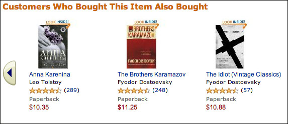
Basket analysis is an alternative mode of learning recommendations. In this mode, our data consists only of what items were bought together; it does not contain any information on whether individual items were enjoyed or not. It is often easier to get this data rather than ratings data as many users will not provide ratings, while the basket data is generated as a side effect of shopping. The following screenshot shows you a snippet of Amazon.com's web page for the book War and Peace, Leo Tolstoy, which is a classic way to use these results:
This mode of learning is not only applicable to actual shopping baskets, naturally. It is applicable in any setting where you have groups of objects together and need to recommend another. For example, recommending additional recipients to a user writing an e-mail is done by Gmail and could be implemented using similar techniques (we do not know what Gmail uses internally; perhaps they combine multiple techniques as we did earlier). Or, we could use these methods to develop an application to recommend webpages to visit based on your browsing history. Even if we are handling purchases, it may make sense to group all purchases by a customer into a single basket independently of whether the items where bought together or on separate transactions (this depends on the business context).
Note
The beer and diapers story
One of the stories that is often mentioned in the context of basket analysis is the "diapers and beer" story. It states that when supermarkets first started to look at their data, they found that diapers were often bought together with beer. Supposedly, it was the father who would go out to the supermarket to buy diapers and then would pick up some beer as well. There has been much discussion of whether this is true or just an urban myth. In this case, it seems that it is true. In the early 1990s, Osco Drug did discover that in the early evening beer and diapers were bought together, and it did surprise the managers who had, until then, never considered these two products to be similar. What is not true is that this led the store to move the beer display closer to the diaper section. Also, we have no idea whether it was really that fathers were buying beer and diapers together more than mothers (or grandparents).
It is not just "customers who bought X also bought Y", even though that is how many online retailers phrase it (see the Amazon.com screenshot given earlier); a real system cannot work like this. Why not? Because such a system would get fooled by very frequently bought items and would simply recommend that which is popular without any personalization.
For example, at a supermarket, many customers buy bread (say 50 percent of customers buy bread). So if you focus on any particular item, say dishwasher soap, and look at what is frequently bought with dishwasher soap, you might find that bread is frequently bought with soap. In fact, 50 percent of the times someone buys dishwasher soap, they buy bread. However, bread is frequently bought with anything else just because everybody buys bread very often.
What we are really looking for is customers who bought X are statistically more likely to buy Y than the baseline. So if you buy dishwasher soap, you are likely to buy bread, but not more so than the baseline. Similarly, a bookstore that simply recommended bestsellers no matter which books you had already bought would not be doing a good job of personalizing recommendations.
As an example, we will look at a dataset consisting of anonymous transactions at a supermarket in Belgium. This dataset was made available by Tom Brijs at Hasselt University. The data is anonymous, so we only have a number for each product and a basket that is a set of numbers. The datafile is available from several online sources (including the book's companion website) as retail.dat.
We begin by loading the dataset and looking at some statistics:
   from collections import defaultdict
from itertools import chain
# file format is a line per transaction
# of the form '12 34 342 5...'
dataset = [[int(tok) for tok in ,line.strip().split()]
        for line in open('retail.dat')]
# count how often each product was purchased:
counts = defaultdict(int)
for elem in chain(*dataset):
    counts[elem] += 1
We can plot a small histogram as follows:
|
# of times bought |
# of products |
|---|---|
|
Just once |
2224 |
|
Twice or thrice |
2438 |
|
Four to seven times |
2508 |
|
Eight to 15 times |
2251 |
|
16 to 31 times |
2182 |
|
32 to 63 times |
1940 |
|
64 to 127 times |
1523 |
|
128 to 511 times |
1225 |
|
512 times or more |
179 |
There are many products that have only been bought a few times. For example, 33 percent of products were bought four or less times. However, this represents only 1 percent of purchases. This phenomenon that many products are only purchased a small number of times is sometimes labeled "the long tail", and has only become more prominent as the Internet made it cheaper to stock and sell niche items. In order to be able to provide recommendations for these products, we would need a lot more data.
There are a few open source implementations of basket analysis algorithms out there, but none that are well-integrated with scikit-learn or any of the other packages we have been using. Therefore, we are going to implement one classic algorithm ourselves. This algorithm is called the Apriori algorithm, and it is a bit old (it was published in 1994 by Rakesh Agrawal and Ramakrishnan Srikant), but it still works (algorithms, of course, never stop working; they just get superceded by better ideas).
Formally, Apriori takes a collection of sets (that is, your shopping baskets) and returns sets that are very frequent as subsets (that is, items that together are part of many shopping baskets).
The algorithm works according to the bottom-up approach: starting with the smallest candidates (those composed of one single element), it builds up, adding one element at a time. We need to define the minimum support we are looking for:
minsupport = 80
Support is the number of times that a set of products was purchased together. The goal of Apriori is to find itemsets with high support. Logically, any itemset with more than minimal support can only be composed of items that themselves have at least minimal support:
  valid = set(k for k,v in counts.items()
          if (v >= minsupport))
Our initial itemsets are singletons (sets with a single element). In particular, all singletons that have at least minimal support are frequent itemsets.
itemsets = [frozenset([v]) for v in valid]
Now our iteration is very simple and is given as follows:
    new_itemsets = []
    for iset in itemsets:
        for v in valid:
            if v not in iset:
          # we create a new possible set
          # which is the same as the previous,
          #with the addition of v
                newset = (ell|set([v_]))
                # loop over the dataset to count the number
                # of times newset appears. This step is slow
                # and not used proper implementation
                c_newset = 0
                for d in dataset:
                   if d.issuperset(c):
                      c_newset += 1
                if c_newset > minsupport:
                    newsets.append(newset)
This works correctly, but is very slow. A better implementation has more infrastructure so you can avoid having to loop over all the datasets to get the count (c_newset). In particular, we keep track of which shopping baskets have which frequent itemsets. This accelerates the loop but makes the code harder to follow. Therefore, we will not show it here. As usual, you can find both implementations on the book's companion website. The code there is also wrapped into a function that can be applied to other datasets.
The Apriori algorithm returns frequent itemsets, that is, small baskets that are not in any specific quantity (minsupport in the code).
Frequent itemsets are not very useful by themselves. The next step is to build association rules. Because of this final goal, the whole field of basket analysis is sometimes called association rule mining.
An association rule is a statement of the "if X then Y" form; for example, if a customer bought War and Peace, they will buy Anna Karenina. Note that the rule is not deterministic (not all customers who buy X will buy Y), but it is rather cumbersome to always spell it out. So if a customer bought X, he is more likely to buy Y according to the baseline; thus, we say if X then Y, but we mean it in a probabilistic sense.
Interestingly, the antecedent and conclusion may contain multiple objects: costumers who bought X, Y, and Z also bought A, B, and C. Multiple antecedents may allow you to make more specific predictions than are possible from a single item.
You can get from a frequent set to a rule by just trying all possible combinations of X implies Y. It is easy to generate many of these rules. However, you only want to have valuable rules. Therefore, we need to measure the value of a rule. A commonly used measure is called the lift. The lift is the ratio between the probability obtained by applying the rule and the baseline:
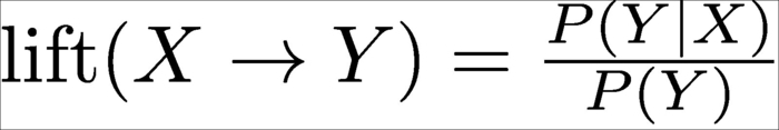
In the preceding formula, P(Y) is the fraction of all transactions that include Y while P(Y|X) is the fraction of transactions that include Y and X both. Using the lift helps you avoid the problem of recommending bestsellers; for a bestseller, both P(Y) and P(X|Y) will be large. Therefore, the lift will be close to one and the rule will be deemed not very relevant. In practice, we wish to have at least 10, perhaps even 100, values of a lift.
Refer to the following code:
def rules_from_itemset(itemset, dataset):
  itemset = frozenset(itemset)
  nr_transactions = float(len(dataset))
  for item in itemset:
           antecendent = itemset-consequent
      base = 0.0
      # acount: antecedent count
        acount = 0.0

    # ccount : consequent count
    ccount = 0.0
    for d in dataset:
      if item in d: base += 1
      if d.issuperset(itemset): ccount += 1
      if d.issuperset(antecedent): acount += 1
    base /= nr_transactions
    p_y_given_x = ccount/acount
    lift = p_y_given_x / base
    print('Rule {0} ->  {1} has lift {2}'
          .format(antecedent, consequent,lift))
This is slow-running code: we iterate over the whole dataset repeatedly. A better implementation would cache the counts for speed. You can download such an implementation from the book's website, and it does indeed run much faster.
Some of the results are shown in the following table:
|
Antecedent |
Consequent |
Consequent count |
Antecedent count |
Antecedent and consequent count |
Lift |
|---|---|---|---|---|---|
|
|
|
|
|
|
|
|
|
|
|
|
|
|
|
|
|
|
|
|
|
Counts are the number of transactions; they include the following:
- The consequent alone (that is, the base rate at which that product is bought)
- All the items in the antecedent
- All the items in the antecedent and the consequent
We can see, for example, that there were 80 transactions of which 1378, 1379l, and 1380 were bought together. Of these, 57 also included 1269, so the estimated conditional probability is 57/80 ≈ 71%. Compared to the fact that only 0.3% of all transactions included 1269 , this gives us a lift of 255.
The need to have a decent number of transactions in these counts in order to be able to make relatively solid inferences is why we must first select frequent itemsets. If we were to generate rules from an infrequent itemset, the counts would be very small; due to this, the relative values would be meaningless (or subject to very large error bars).
Note that there are many more association rules that have been discovered from this dataset: 1030 datasets are required to support at least 80 minimum baskets and a minimum lift of 5. This is still a small dataset when compared to what is now possible with the Web; when you perform millions of transactions, you can expect to generate many thousands, even millions, of rules.
However, for each customer, only a few of them will be relevant at any given time, and so each costumer only receives a small number of recommendations.
There are now other algorithms for basket analysis that run faster than Apriori. The code we saw earlier was simple, and was good enough for us as we only had circa 100 thousand transactions. If you have had many millions, it might be worthwhile to use a faster algorithm (although note that for most applications, learning association rules can be run offline).
There are also methods to work with temporal information leading to rules that take into account the order in which you have made your purchases. To take an extreme example of why this may be useful, consider that someone buying supplies for a large party may come back for trash bags. Therefore it may make sense to propose trash bags on the first visit. However, it would not make sense to propose party supplies to everyone who buys a trash bag.
You can find Python open source implementations (a new BSD license as scikit-learn) of some of these in a package called pymining. This package was developed by Barthelemy Dagenais and is available at https://github.com/bartdag/pymining.