A very convenient way to get a quick impression of how the songs of the diverse genres "look" like is to draw a spectrogram for a set of songs of a genre. A spectrogram is a visual representation of the frequencies that occur in a song. It shows the intensity of the frequencies on the y axis in the specified time intervals on the x axis; that is, the darker the color, the stronger the frequency is in the particular time window of the song.
Matplotlib provides the convenient function specgram() that performs most of the under-the-hood calculation and plotting for us:
>>> import scipy
>>> from matplotlib.pyplot import specgram
>>> sample_rate, X = scipy.io.wavfile.read(wave_filename)
>>> print sample_rate, X.shape
22050, (661794,)
>>> specgram(X, Fs=sample_rate, xextent=(0,30))
The wave file we just read was sampled at a sample rate of 22,050 Hz and contains 661,794 samples.
If we now plot the spectrogram for these first 30 seconds of diverse wave files, we can see that there are commonalities between songs of the same genre:
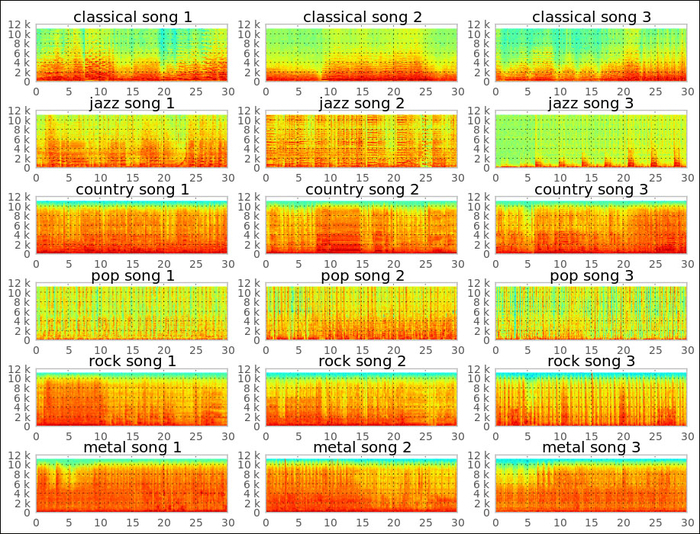
Just glancing at it, we immediately see the difference in the spectrum between, for example, metal and classical songs. While metal songs have high intensity over most of the frequency spectrum all the time (energize!), classical songs show a more diverse pattern over time.
It should be possible to train a classifier that discriminates at least between metal and classical songs with an accuracy that is high enough. Other genre pairs such as country and rock could pose a bigger challenge, though. This looks like a real challenge to us, as we need to discriminate not just between two classes, but between six. We need to be able to discriminate between all six reasonably well.
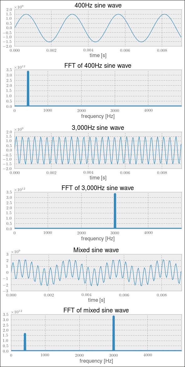
Our plan is to extract individual frequency intensities from the raw sample readings (stored in X earlier) and feed them into a classifier. These frequency intensities can be extracted by applying the Fast Fourier Transform (FFT). As the theory behind FFT is outside the scope of this chapter, let us just look at an example to get an intuition of what it accomplishes. Later on, we will then treat it as a black box feature extractor.
For example, let us generate two wave files, sine_a.wav and sine_b.wav, which contain the sound of 400 Hz and 3,000 Hz sine waves. The Swiss Army Knife, sox, mentioned earlier is one way to achieve this:
$ sox --null -r 22050 sine_a.wav synth 0.2 sine 400
$ sox --null -r 22050 sine_b.wav synth 0.2 sine 3000
The charts in the following screenshot show the plotting of the first 0.008 seconds. We can also see the FFT of the sine waves. Not surprisingly, we see a spike at 400 and 3,000 Hz below the corresponding sine waves.
Now let us mix them both, giving the 400 Hz sound half the volume of the 3,000 Hz one:
$ sox --combine mix --volume 1 sine_b.wav --volume 0.5 sine_a.wav sine_mix.wav
We see two spikes in the FFT plot of the combined sound, of which the 3,000 Hz spike is almost double the size of the 400 Hz one:
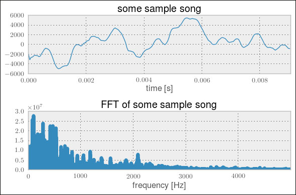
For real music, we can quickly see that the FFT looks not as beautiful as in the preceding toy example: