We have already learned that FFT is pointing us in the right direction, but in itself it will not be enough to finally arrive at a classifier that successfully manages to organize our scrambled directory containing songs of diverse music genres into individual genre directories. We somehow need a more advanced version of it.

At this point, it is always wise to acknowledge that we have to do more research. Other people might have had similar challenges in the past and already found out new ways that might also help us. And indeed, there is even a yearly conference only dedicated to music genre classification organized by the International Society for Music Information Retrieval (ISMIR). Apparently, Automatic Music Genre Classification (AMGC) is an established subfield of Music Information Retrieval (MIR). Glancing over some of the AMGC papers, we see that there is a bunch of work targeting automatic genre classification that might help us.

One technique that seems to be successfully applied in many of those works is called Mel Frequency Cepstral Coefficients (MFCC). The Mel Frequency Cepstrum (MFC) encodes the power spectrum of a sound. It is calculated as the Fourier transform of the logarithm of the signal's spectrum. If that sounds too complicated, simply remember that the name "cepstrum" originates from "spectrum", with the first four characters reversed. MFC has been successfully used in speech and speaker recognition. Let's see whether it also works in our case.

We are in a lucky situation where someone else has already needed exactly what we need and published an implementation of it as the Talkbox SciKit. We can install it from https://pypi.python.org/pypi/scikits.talkbox. Afterwards, we can call the mfcc() function, which calculates the MFC coefficients as follows:

>>>from scikits.talkbox.features import mfcc
>>>sample_rate, X = scipy.io.wavfile.read(fn)
>>>ceps, mspec, spec = mfcc(X)
>>> print(ceps.shape)
(4135, 13)

The data we would want to feed into our classifier is stored in ceps, which contains 13 coefficients (the default value for the nceps parameter of the mfcc() function) for each of the 4135 frames for the song with the filename fn. Taking all of the data would overwhelm our classifier. What we could do instead is to do an averaging per coefficient over all the frames. Assuming that the start and end of each song are possibly less genre-specific than the middle part of it, we also ignore the first and last 10 percent:

x = np.mean(ceps[int(num_ceps*1/10):int(num_ceps*9/10)], axis=0)

Sure enough, the benchmark dataset that we will be using contains only the first 30 seconds of each song, so that we would not need to cut off the last 10 percent. We do it nevertheless, so that our code works on other datasets as well, which are most likely not truncated.

Similar to our work with FFT, we certainly would also want to cache the once-generated MFCC features and read them instead of recreating them each time we train our classifier.

This leads to the following code:

def write_ceps(ceps, fn):
    base_fn, ext = os.path.splitext(fn)
    data_fn = base_fn + ".ceps"
    np.save(data_fn, ceps)
    print("Written %s" % data_fn)

def create_ceps(fn):
    sample_rate, X = scipy.io.wavfile.read(fn)
    ceps, mspec, spec = mfcc(X)
    write_ceps(ceps, fn)

def read_ceps(genre_list, base_dir=GENRE_DIR):
    X, Y = [], []
    for label, genre in enumerate(genre_list):
        for fn in glob.glob(os.path.join(
base_dir, genre, "*.ceps.npy")):
            ceps = np.load(fn)
            num_ceps = len(ceps)
X.append(np.mean(
ceps[int(num_ceps*1/10):int(num_ceps*9/10)], axis=0))
y.append(label)

    return np.array(X), np.array(y)

We get the following promising results, as shown in the next screenshot, with a classifier that uses only 13 features per song:

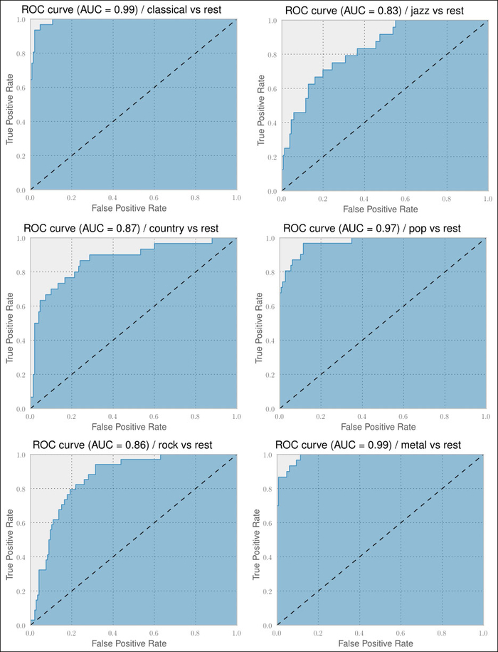
The classification performance for all genres has improved. Jazz and metal are even at almost 1.0 AUC. And indeed, the confusion matrix in the following plot also looks much better now. We can clearly see the diagonal showing that the classifier manages to classify the genres correctly in most of the cases. This classifier is actually quite usable to solve our initial task:

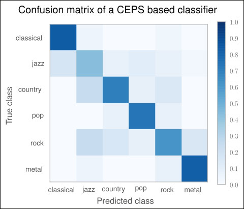
If we would want to improve on this, this confusion matrix quickly tells us where to focus on: the non-white spots on the non-diagonal places. For instance, we have a darker spot where we mislabel jazz songs as being rock with considerable probability. To fix this, we would probably need to dive deeper into the songs and extract things, for instance, drum patterns and similar genre-specific characteristics. Also, while glancing over the ISMIR papers, you may have also read about so-called Auditory Filterbank Temporal Envelope (AFTE) features, which seem to outperform the MFCC features in certain situations. Maybe we should have a look at them as well?

The nice thing is that being equipped with only ROC curves and confusion matrices, we are free to pull in other experts' knowledge in terms of feature extractors, without requiring ourselves to fully understand their inner workings. Our measurement tools will always tell us when the direction is right and when to change it. Of course, being a machine learner who is eager to learn, we will always have the dim feeling that there is an exciting algorithm buried somewhere in a black box of our feature extractors, which is just waiting for us to be understood.