Chapter 37. Interacting with Other Office Applications

In this chapter

Pasting Excel Data to Microsoft OneNote 1006

Pasting Excel Data to PowerPoint 1009

Creating Tables in Excel and Pasting to Word 1011

Pasting Word Data to an Excel Text Box 1012

Using Excel Data in a Word Mail Merge 1013

Building a Pivot Table from Access Queries 1016

After authoring a worksheet in Excel, you might need to include its information in a PowerPoint presentation or a Word document. Or you might want to add portions of your spreadsheet in your OneNote workbook (assuming that your version came with OneNote). The collaborative nature of Office 2007 applications allow you to do this with ease.

Although the core Office 2007 applications offer themes and the new ribbon interface, they still do not play perfectly well together. The Microsoft marketing machine would have you believe that themes are designed to make all your documents, from Excel to Word to PowerPoint, look similar. However, after data is been pasted from Excel to another application, changes to the theme do not carry through. I would expect this will be one of the areas that Microsoft works on for Office 14.

In certain cases, you can utilize Excel data without ever opening the Excel file. If you have a list of addresses in Excel, you can access that list when doing a mail merge in Microsoft Word 2007. Excel can receive data from other Office applications. For example, you might author body copy in Word and then copy it to a text box in Excel. Data from Access can also be used as the source data for an external query in Excel or even for a pivot table.

Pasting Excel Data to Microsoft OneNote

Microsoft OneNote 2007 is being bundled as part of Microsoft Office 2007 for the Student and Home editions. This product was introduced in Office 2003 but was never bundled with any version of Office. It is a fantastic product but a product that not many people were willing to spend $99 to buy. Now that OneNote is bundled with some versions of Office, it will finally get the exposure needed to allow more people to gravitate toward its ability to organize notes in one place.

In the initial release of OneNote, the ability to present tabular data was dismal. OneNote 2007 finally does an adequate job of presenting tabular data from Excel. OneNote offers several formatting options to choose from after pasting Excel data to OneNote. These options are contrasted here.

Figure 37.1 shows a region in an Excel worksheet that has been formatted with various built-in styles.

Figure 37.1. You select a region of the worksheet that you would like to copy to OneNote.

To copy an Excel region to OneNote, you follow these steps:

1. Select the range in Excel.
2. Press Ctrl+C to copy the selected range to the Clipboard.
3. Switch to Microsoft OneNote 2007.
4. Click in the approximate location where you would like the data to be pasted.
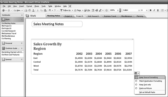
5. Use Edit, Paste or Ctrl+V to paste the data. A Paste Options drop-down appears to the right of the pasted range.
6. Click the arrow next to the Paste Options drop-down. The choices follow:

   • Keep Source Formatting: This option is shown in Figure 37.2. The color fills are not present, and the word wrap from the former Cell A1 is a little bizarre, but you still see the basic look and feel of the worksheet.

   Figure 37.2. When Keep Source Formatting is selected, the text colors and sizes are pasted from Excel.

   

   • Match Destination Formatting: Figure 37.3 shows the results of choosing Match Destination Formatting from the Paste Options drop-down. All the fonts are pasted at the same size and color.

   Figure 37.3. When Match Destination Formatting is selected, the text colors are kept, but the sizes are made uniform to match the current font size.

   

   • Keep Text Only: This option generally looks horrible with data from Excel. It should be avoided.

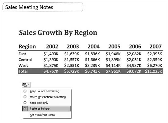
   • Paste as Picture: This option keeps the exact look of the document from Excel, including the color fills, as shown in Figure 37.4. The only problem with this format is that you cannot use the clipboard to copy numbers from the picture.

   Figure 37.4. Convert the pasted selection to a table to produce an exact representation of the formatting from Excel.

   

7. Choose one of the options from the drop-down to complete the paste.

The final option in OneNote is to create a screen clipping to be pasted to OneNote. This option produces an exact screen capture of a region of the worksheet. To do this, you follow these steps:

1. In Excel, arrange the window so that you can see all the data and elements that need to be copied to OneNote.
2. Switch to OneNote. (Do not stop at any other applications first because the screen clipping utility goes to the last application window active before the command.) Position the cursor at a point where you would like the screen clipping to be pasted.
3. Select Insert, Screen Clipping. The OneNote window is hidden, and you see a grayed-out rendering of the last active application.
4. Using your mouse, drag a rectangle around the area you want to copy. As you drag, the rectangular area switches from grayed out to color, as shown in Figure 37.5.

   Figure 37.5. After invoking screen clipping from OneNote, you draw a rectangle to indicate the area to be copied.

   

5. When you release the mouse, the screen clipping is transferred to OneNote. OneNote adds a footer indicating the date and time of the clipping.

Support for tables has dramatically improved in OneNote 2007. Whereas pasting Excel tables to OneNote 2003 was disappointing, there are now three viable options for pasting Excel data to OneNote.

Pasting Excel Data to PowerPoint

The process of copying data from Excel to PowerPoint is simpler in Excel 2007 than in previous versions.

By default, if you copy a range and paste to PowerPoint, the range is pasted in HTML format. This means that none of the formulas are live.

In prior versions of Office, Excel data was pasted to PowerPoint as an Excel object. This meant that even if you pasted 20 cells, the entire workbook was lurking behind the 20 cells and accessible to anyone who could open the PowerPoint file.

Using Excel Tables in PowerPoint

To copy data from Excel to PowerPoint, you follow these steps:

1. Prepare a blank slide in PowerPoint that is ready to accept the data from Excel.
2. Open the desired Excel workbook.
3. Select the range to be copied.
4. Press Ctrl+C to copy the selected range.
5. Switch back to PowerPoint.
6. From the Home ribbon, choose Paste.
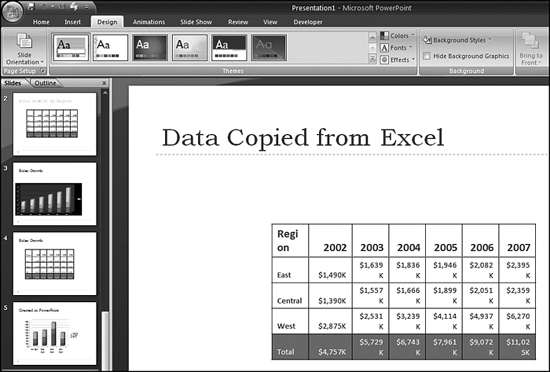
7. If some columns are not wide enough after the paste (see Figure 37.6), resize the table to be slightly larger and drag the column borders to allow the contents to fit.

Figure 37.6. Tables might need to be resized after being pasted to PowerPoint.

This method uses the default paste method, which is now Paste as HTML. If you instead prefer to go back to the old method, you choose Paste, Paste Special, Microsoft Office Excel Worksheet Object.

Using Excel Charts in PowerPoint

The process of copying charts from Excel to PowerPoint works much better than the process of copying tables from Excel. The resulting chart is completely editable in PowerPoint. In addition, changes to the slide theme change the look and feel of the chart.

To copy a chart to PowerPoint, you follow these steps:

1. Prepare a blank slide in PowerPoint that is ready to accept the data from Excel.
2. Open the desired Excel workbook.
3. Select the chart to be copied.
4. Press Ctrl+C to copy the selected chart.
5. Switch back to PowerPoint.
6. From the Home ribbon, choose Paste.

As shown in Figure 37.7, the chart is pasted to the slide. You can resize the chart to fill the area on the slide.

Figure 37.7. Charts pasted into PowerPoint have the same look and feel as in Excel, as well as the same user interface tabs on the ribbon.

When the chart is selected in PowerPoint, three new ribbon tabs offer the same chart experience as is available in Excel.

Creating Tables in Excel and Pasting to Word

Microsoft Word is excellent for typing body text. When you need to start creating tables in Word, however, the program is a bit confusing. If you are more comfortable with Excel than Word, it makes sense to switch to Excel, create and format a table, and then paste the table back to the Word document. This gives you better control over column widths, plus the possibility to provide formulas for calculating some of the content of the table.

To create a table for Word, using Excel, you follow these steps:

1. Position the insertion cursor in Word at a point where the table should go.
2. Switch to Excel and open a blank document.
3. Type the data in columns in Excel.
4. If you use formulas to build rows of the table, it is best to convert the formulas to values before copying to Word. To do so, select the formulas and press Ctrl+C to copy. Then select Home, Paste, Paste Values.
5. If you have chosen a theme in Word, choose the identical theme in Excel.
6. Select the table and then select the Cells section of the Home ribbon and choose Format, Width, AutoFit Selection.
7. Optionally, apply a table format as shown in Chapter 8.
8. Select the table in Excel and then press Ctrl+C to copy.
9. Switch to Word.
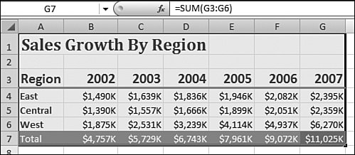
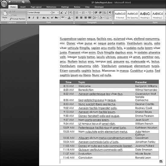
10. From the Home ribbon, choose Paste. An HTML representation of the table is pasted into Word. The column widths, alignment, font, font color, and fill copy perfectly from Excel, as shown in Figure 37.8.

Figure 37.8. An Excel range copied to Word builds a perfect table, with all the right column widths.

Pasting Word Data to an Excel Text Box

Although Excel is great at handling tables of numbers, it does not have the editing tools needed to make it easy to handle body copy as well as in Word. If you want to be able to type paragraphs of text without needing to judge the length of each line, you should use Word to prepare the text and then paste it to a text box in Excel. You can follow these steps to build a section of body copy for use in Excel:

1. Switch to Microsoft Word and open a blank document.
2. Type the text. Use any formatting you like, such as underlining, bold, italics, font size, font changes, and so on.
3. Select the text in Word.
4. Press Ctrl+C to copy the selected text.
5. Switch to Excel.
6. On the Insert ribbon, choose Text, Text Box.
7. Drag in the worksheet to define the shape of the text box.
8. When you release the mouse, the insertion point is at the start of the text box. Press Ctrl+V to paste.
9. By default, text boxes have a visible border. To remove the border, select Drawing Tools Format, Shape Styles, Shape Outline, No Outline.
10. If you need to resize or further format the text, select the text in the text box. The mini toolbar appears. If desired, change font size, style, and so on.

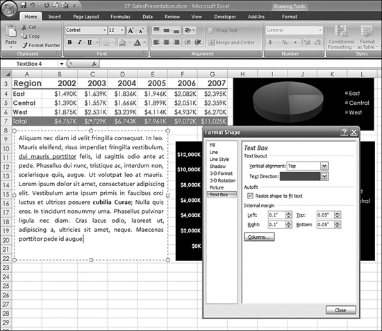
If you need to fine-tune the text box, follow these steps:

1. Click outside the text box.
2. Right-click the text box and choose Format Shape. The Format Shape dialog appears.
3. In the Format Shape dialog, select the Text Box category.
4. Select an internal margin, select text alignment, add columns, or resize the shape to fit the text, as shown in Figure 37.9.

Figure 37.9. After copying Word text to a text box, you can use the formatting tools to fine-tune the text box.

Using Excel Data in a Word Mail Merge

Word’s mail merge tools allow you to create a printed form letter that is customized to each person in an Excel list of names. For the best results, your Excel table should include columns for first name, last name, address line 1, address line 2, city, state or province, and zip or postal code.

You follow these steps to perform a mail merge in Word using Excel data:

1. Prepare your data in Excel. Include headings for each column. Do not include any blank columns or entirely blank rows.
2. To simplify the mail merge, select the range and press Ctrl+T to convert the range to a table. Be sure to specify that the table has headers.
3. Save and close the Excel workbook.
4. Open Microsoft Word.
5. Leave a few blank lines at the top for the address block and greeting.
6. Type the rest of the letter.
7. Choose Mailings, Start Mail Merge, Start Mail Merge, Step by Step Mail Merge. A Mail Merge task pane appears on the right side of the screen.
8. By default, Step 1 of the task pane indicates that you are producing a letter. At the bottom of the task pane, click the hyperlink for Next.
9. In Step 2 of the task pane, choose to use the current document. Click Next.
10. In Step 3 of the task pane, choose Use an Existing List and then choose Select List. The Select Data Source dialog appears.
11. Browse to your Excel file and click Open. The Select Table dialog appears.
12. In the Select Table dialog, Word selects the table in your document. Click OK to confirm. Word displays the Mail Merge Recipients dialog.
13. If desired, choose to filter or sort the list, as shown in Figure 37.10. Click OK to continue.

    Figure 37.10. You preview the records from Excel in this dialog.

    

14. In the Mail Merge taskbar, click Next.
15. In Step 4 of the task pane, the instructions say to write your letter. This is the step where you insert placeholders from the Excel file. In the Mailings ribbon, choose Write & Insert Fields, Match Fields. The Match Fields dialog appears.
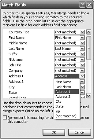
16. Depending on your headings, the IntelliSense might match your headings to the proper fields. Browse through the fields to make sure all your fields have been matched. If you know that there is a field in your Excel file that does not appear on the right side of the Match Fields dialog, use the drop-down to map the Excel column to the proper field in Word, as shown in Figure 37.11. Word has categories for items that you might not have included in your data. It is okay if you don’t have a match for every possible Word field. However, make sure that Word knows about every field in your data.

    Figure 37.11. Before attempting to insert fields, make sure that Word has correctly identified any name or address fields in your data.

    

17. Position the insertion cursor where the address block should go. In the Mailings ribbon, click Address Block. Excel displays the Insert Address Block dialog. You can preview the various addresses here. If there are problems, use the Match Fields dialog to rematch the fields.
18. Click OK to close the Insert Address Block dialog. Words adds a field code to your document that looks like <<AddressBlock>>. The insertion point remains on the same line as the address block, so press Enter to move to the next line.
19. From the Mailings ribbon, choose Greeting Line. In the Insert Greeting Line dialog that appears, build your greeting line. The three drop-downs allow you to specify “Dear” or “To,” various forms of the person’s name, and a comma or a colon. Click OK.
20. If desired, include fields from the Excel file in the body of your letter. For example, a marketing letter might refer to the person’s city in the body of the letter. Position the cursor at the appropriate place in the letter. From the ribbon, choose the Insert Merge Field drop-down. From the list, select the appropriate field from the Excel file.
21. In the Mail Merge task pane, select Next to proceed to Step 5 of the task pane.
22. In Step 5 of the task pane, Word previews the letter for the first recipient. You can format the address block at this point. You can also use the >> button on the taskbar to browse through the names.
23. In the task pane, click Next.
24. In Step 6 of the task pane, choose to print or edit individual letters, if needed. If you choose Print, Word sends one letter to the printer for each row in your Excel list. If you choose Edit Individual Letters, Excel creates a new document with a new page for each document.

Using Mail Merge in Word is a quick way to send customized letters to many recipients at once. The Mailings toolbar has options for creating envelopes and mailing labels as well. The steps for both of these document types are similar to those just provided for mail merges.

Building a Pivot Table from Access Queries

Microsoft Access is the database component of Microsoft Office. It is included in the Professional versions of Office 2007 but not with the Home edition of Microsoft Office.

Before Excel 2007, many people occasionally encountered Access when they had more than 65,536 rows of data. Now that Excel can handle 1.1 million rows, there will be less casual use of Access.

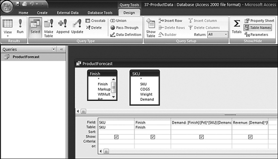
Access is a relational database. This means that relationships can be defined between multiple tables, and these tables can be joined together in a query. In Figure 37.12, a query is defined in Access to join two tables together. Calculated fields can calculate values from fields in each table.

Figure 37.12. This query joins multiple Access tables.

To use this data in an Excel pivot table, you follow these steps:

1. Ensure that the Access database is saved in a trusted location. If you are unsure of trusted locations, choose the Office icon and then select Excel Options, Trust Center, Trust Center Settings, Trusted Locations. If the location of the Access database is not in the list of trusted locations, choose Add New Location.
2. In Excel, choose Insert, Tables, PivotTable. The Create Pivot Table dialog appears.
3. In the Create Pivot Table dialog, choose Use an External Data Source.
4. Click the Choose Connection button. The Existing Connections dialog appears.
5. In the Existing Connections dialog, click Browse for More.
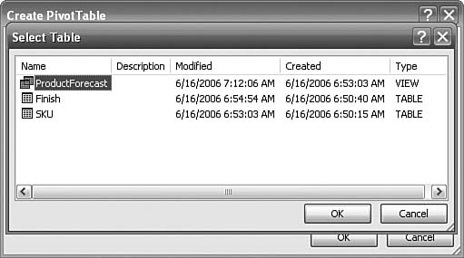
6. Browse to and select your database. Click Open. The Select Table dialog appears.
7. As shown in Figure 37.13, the Select Table dialog offers all the available tables and views in the Access database. Note that queries in Access are shown as views. Click the desired view and click OK.

   Figure 37.13. Excel shows a list of available tables and queries.

   

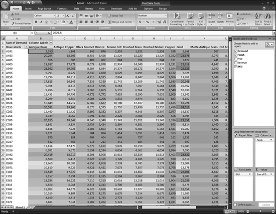
8. Click OK to create the pivot table. The Access data is now available for querying. You can choose pivot table fields as described in Chapter 10, “Using Pivot Tables to Analyze Data.”

The advantage of this method is that the data never has to be copied to Excel. In this case, two relatively small Access tables are joined into a larger query result. As shown in Figure 37.14, the pivot table presents results from the query without having to store the detailed data in Excel.

Figure 37.14. This pivot table creates a summary from thousands of virtual rows of data in Access without ever storing that data in the workbook.