
Appendix 9
A MINISCULE INTRODUCTION TO FRACTALS
The person most often associated with the discovery of fractals (and rightly so) is the mathematician Benoit B. Mandelbrot. Indeed, one doesn’t need to be the proverbial rocket scientist to see why the Mandelbrot set is so named (for details of this amazing set, just Google the name!). The mathematics underlying the structure of fractals (geometric measure theory), however, had been developed long before the “computer revolution” made possible the visualization of such complicated mathematical objects. In the 1960s Mandelbrot pointed out some interesting but very surprising results in a paper entitled “How long is the coastline of Britain?” published posthumously by the English meteorologist Lewis Fry Richardson. That author had noticed that the measured length of the west coast of Britain depended heavily on the scale of the map used to make those measurements: a map with scale 1:10,000,000 (1 cm being equivalent to 100 km) has less detail than a map with scale 1:100,000 (1 cm equivalent to 1 km). The more detailed map, with more “nooks and crannies,” gives a larger value for the coastline. Alternatively, one can imagine measuring a given map with smaller and smaller measuring units, or even walking around the coastline with smaller and smaller graduations on our meter rule. Of course this presumes that at such small scales we can meaningfully define the coastline, but naturally this process cannot be continued indefinitely due to the atomic structure of matter. This is completely unlike the “continuum” mathematical models to which we have referred in this book, and in which there is no smallest scale.
Richardson also investigated the behavior with scale for other geographical regions: the Australian coast, the South African coast, the German Land Frontier (1900), and the Portugese Land Frontier. For the west coast of Britain in particular, he found the following relationship between the total length s in km and the numerical value a of the measuring unit (in km, so a is dimensionless):
where s1 is the length when a = 1. Clearly, as a is reduced, s increases! If the measuring unit were one meter instead of one km, the value of s would increase by a factor of about 4.6 according to this model. Clearly, the concept of length in this context is rather amorphous; is there a better way of describing the coastline? Can we measure the “crinkliness” or “roughness” or “degree of meander” or some other such quantity? Mandelbrot showed that the answer to this question is yes, and the answer is intimately connected with a generalization of our familiar concept of “dimension.” That is the so-called topological dimension, expressed in the natural numbers 0, 1, 2, 3, . . . (there is no reason to stop at three, by the way). It turns out that the concept of fractal dimension used by Mandelbrot (the Hausdorff-Besicovich dimension), being a ratio of logarithms, is not generally an integer. Mandelbrot defines a fractal as “a set for which the Hausdorff-Besicovich dimension strictly exceeds the topological dimension.”
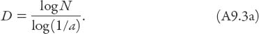
Consider the measurement of a continuous curve by a “measuring rod” of length a. Suppose that it fits N times along the length of the curve, so that the measured length L = Na. Obviously then, N = L/a is a function of a, that is, N = N(a). Thus if a = 1, N(1) = L. Similarly, if a = 1/2, N(1/2) = 2L, N(1/3) = 3L, and so on. For fractal curves, N = La−D, where D > 1 in general, and it is called the fractal dimension. This means that making the scale three times as large (or a one third of the size it was previously) may lead to the measuring rod fitting around the curve more than three times the previous amount. This is because if N(1) = L as before,
![]()
In what follows below we shall use unit length, L = 1 when a = 1 without loss of generality. Given that N = a−D it follows that
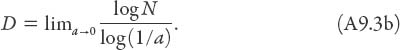
More precisely, Mandelbrot used the definition of the fractal dimension as
If this has the same value at each step, then the former definition is perfectly general. Let us apply the definition to what has come to be called the Koch snowflake curve. The basic iteration step is to take each line segment or side of an equilateral triangle, remove the middle third, and replace it by two sides of an equilateral triangle (each side of which is equal in length to the middle third), so now it is a “Star of David.” Each time this procedure is carried out the previous line segment is increased in length by a factor 4/3. Thus a = 1/3 and N = 4 (there now being four smaller line segments in place of the original one), so
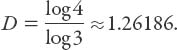
The limiting snowflake curve (a → 0) thus “intrudes” a little into the second dimension; this intrusion is indicated by the degree of “meander” as expressed by the fractal dimension D. This curve is everywhere continuous but nowhere differentiable! The existence of such curves, continuous but without tangents, was first demonstrated well over a century ago by the German mathematician Karl Weierstrass (1815–1897), and this horrified many of his peers. Physicists, however, were more welcoming; Ludwig Boltzmann (1844–1906) wrote to Felix Klein (1849–1925) in January 1898 with the comment that such functions might well have been invented by physicists because there are problems in statistical mechanics “that absolutely necessitate the use of non-differentiable functions.” He had in mind, no doubt, Brownian motion (this is the constant and highly erratic movement of tiny particles (e.g., pollen) suspended in a liquid or a gas, or on the surface of a liquid).
Consider next the box-fractal: this is a square, in which the basic iteration is to divide it into 9 identical smaller squares and remove the middle squares from each side, leaving 5 of the original 9. It is readily seen that a = 1/3 and N = 5, so
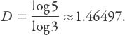
The Sierpinski triangle is any triangle for which the basic iteration is to join the midpoints of the sides with line segments and remove the middle triangle. Now a = 1/2 and N = 3, so
These fractals penetrate increasingly more into the second dimension. We will mention two more at this juncture: the Menger sponge and Cantor dust. For the former, we do in three dimensions what was done in two for the box fractal. Divide a cube into 27 identical cubes and “push out” the middle ones in each face (and the central one). Now it follows that a = 1/3 and N = 20 (seven smaller cubes having been removed in the basic iterative step), so in the limit of the requisite infinite number of iterations
(intruding well into the third dimension). Now for Cantor dust: what is that? Take any line segment and remove the middle third; this is the basic iteration. In the limit of an infinity of such iterations for which a = 1/3 and N = 2, it follows that
which is obviously less than one. Quite amazing.