Chapter 17

THE AXIOMATIC CITY

In this chapter we try to be a little more formal by defining axioms for an equilibrium model of a circular city. By using the word “equilibrium” here, we mean that the “forces” attracting people to live in the city are balanced at every point by the “forces” that “repel” them. Of course, there are no forces in the physical sense of that word, but by analogy with the balance between gravity and pressure gradients in stars it is possible to suggest certain forms of “coercion” that persuade individuals to live exactly where they do. Let’s get started.

X = ρ(r): CIRCLES IN THE CITY

We make the following assumptions (or equivalently, define the following axioms):

  I. The population is distributed with circular symmetry in the plane, with radial “civic” population density ρ(r).

  II. There is an inward cohesive force inducing citizens to relocate nearer the city center; this is because of the desirability of being near work and shopping locations, with lower transportation costs, etc.

 III. There is an outward dispersive force, specifically a housing pressure gradient, inducing citizens to relocate farther from the city center; this is because of higher rental and housing costs in the central regions, etc. This assumption may not be entirely realistic for many modern cities (but we proceed with it nonetheless).

 IV. The civic mass M(r) is the total amount of “civic matter” interior to r.

  V. The cohesive pressure C(r) is similar to a two-dimensional “gravitational attraction” in the plane. In a similar manner, it can be written in terms of the civic mass and distance from the city center.

 VI. The housing pressure P(r) has a power-law dependence on the population density, namely P(r) = A(ρ(r))^γ where A and γ are positive constants. (Recall that this power law dependence was mentioned in Chapter 3.)

VII. The city is said to be in equilibrium if at each point within it the two opposing pressure gradients balance one another. This means that there is no net inducement for the populace to move elsewhere (clearly unusual in practice!).

The model we shall develop is essentially a two-dimensional version of the pressure balance equation for stellar equilibrium, as suggested above. Who would have thought that two such different topics could be so intimately connected? Suppressing our astonishment, let’s combine these assumptions in mathematical form by referring to Figure 17.1. The civic mass is readily seen to be

where ξ is a dummy radial variable. Consider a small change δC in C corresponding to a small increment δM in a radial direction; from Figure 17.1 we have that δM ≈ ρδr. Since we are assuming a gravity-type attraction, we posit that

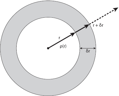
Figure 17.1. Schematic geometry for the civic mass integral in equation (17.1).

In this equation, the “civic coercion” constant k and α are also positive constants; for strictly two-dimensional “gravitational attraction” α = 1, but we shall keep it arbitrary for most of this chapter. Assuming further that C(r) is differentiable, we find that, using the standard limiting procedure, that

The civic pressure gradient is from the higher housing-cost pressures in the central city regions to the lower pressure regions farther out. The cohesive pressure is higher in these external regions, and so the corresponding pressure gradient is in the opposite direction. For a city in equilibrium, therefore, the following equation must be satisfied:

From equations (17.2) and (17.3) we find that

There are several general properties of our “city” that can be established from this equilibrium equation. For example, it follows trivially that the rental gradient P′(r) vanishes at any noncentral location where the population density ρ(r) = 0. In particular, the following exercise is left to the reader:

Exercise: Prove the following results:

(a) The central rental gradient P′(0) is always zero at an equilibrium provided α < 2. (Hint: use L’Hôpital’s rule.)

(b) The quantity decreases monotonically outward for r > 0.

(c) For all r, and

(d) If the rental P(r) = 0 for some radius r = R, then the central rental P(0) satisfies

Further results can be found by using the following definition of a mean rental (r):

Exercise: Prove that if the central rental P(0) ≥ 0, then and hence that

(Hint: integrate by parts twice.)

Now we proceed to look at some more specific city models. We set γ = 2 in “Axiom” VI and write equation (17.4) in terms of the population density ρ(r) to obtain

If we perform a differentiation and define β² = A/πk, then we have

This expression can be rearranged in the form

This equation is related to the well-known Bessel equation of order , namely.

The constant may take on any value, but is often an integer. A bounded solution to this equation satisfying the condition y′(0) = 1 is y = J_v(x), where J_v(x) is a Bessel function of the first kind of order . Consequently, the corresponding solution of equation (17.6) can be shown to be

In this expression ρ(0) is the central population density and = |(1 − α)/(3 − α)|. It will be left as an exercise for the reader to verify this result. Note that if α = 3, the original differential equation (17.6) reduces to Euler’s equation, solutions for which may be found by seeking them in the form ρ(r) ∝ r^m and solving the resulting quadratic equation for m. Only solutions for which the real part of m is positive will be appropriate for a city containing the origin, but for an annular city, all solutions are in principle permitted.

Exercise: Verify by direct construction that (17.8) is a solution to (17.6).

(Hint: let ρ(r) = r^(1−α)/2z(r) and then make a change of independent variable, t = r^(3−α)/2.)

Such idealized “cities” can be referred to as “Bessel cities” for obvious reasons. When α = 1, the solution (17.8) reduces to the simple form ρ(r) = ρ(0) J₀(r/β), and when α = 2 the solution is . From the definition of housing rental the corresponding expressions for P(r) are proportional to the squares of these solutions; they are illustrated in Figure 17.2. The model for α = 2 has the disadvantage that, unlike the case for α = 1, the gradients ρ′(0) and P′(0) at the center are not zero. While this is not a major problem, this model does not have these “nice” properties enjoyed by the other one.

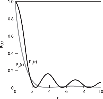
Figure 17.2. P₁(r) (solid line) is the square of the solution (17.8) for α = 1, ρ₀ = 1, and β = 1 (for simplicity). P₂(r) (gray line) is the square of the solution (17.8) for α = 2, ρ₀ = 1, and β = 1.

For Bessel cities, both the density and rental are oscillatory and vanish infinitely often as the distance from the center increases indefinitely. Furthermore, the model predicts that the population density can become negative. Obviously this cannot be the case in reality, so it makes sense to define a finite Bessel city by truncating the model at the first zero of the corresponding Bessel function. It is interesting to note that in his α = 1 models, Amson (1972, 1973) identifies the positive but ever-decreasing peaks in the Bessel function as “satellite town belts” surrounding a central city, with the regions of negative density identified as greenbelt regions. If the first zero of J₀(r/β) occurs at r = R₁, the area of this can be called the central area, with central population M(R₁). The zeros of Bessel functions are tabulated and available online. Since the first zero of J₀(x) occurs when x ≈ 2.405, it follows that R₁ ≈ 2.405β = 2.405(A/πk)^1/2. Hence the central area is

From this simple result we see that it depends directly on the rental coefficient A and inversely on the coercion coefficient k, but is independent of the central density ρ(0). It can also be shown that for given values of A and k the central rental P(0) varies as the square of the central population.