
Chapter 6
SUMMER IN THE CITY

Question: How many squirrels live in Central Park?
Central Park in New York City runs from 59th Street to 110th Street [6]. At 20 blocks per mile, this is 2.5 miles. Central Park is long and narrow, so we will estimate its width at about 0.5 mile. This gives an area of about 1 square mile or about 2 square kilometers.
It’s difficult to estimate the number of squirrels in that large an area, so let’s break it down and think of the area of an (American) football field (about 50 yards × 100 yards). There will be more than 1 and fewer than 1000 squirrels living there, so we choose the number geometrically between 1 and 1000, or 30 (using the Goldilocks principle again).
This is where the metric system comes in handy. One kilometer (1000 m or about 1100 yards; we’ll round down to 1000 yards) is the length of ten football fields and the width of twenty. This means that there are 200 football fields in a square kilometer. Now the number of squirrels in Central Park is about N = (2 km2) × (200 football fields/(km2)) × (30 squirrels/football field) = 12,000 ≈ 104. That’s enough squirrels for even the most ambitious dog to chase!
X = X : SUNBATHING IN THE CITY
It’s a lovely weekend and you decide to “catch some rays” in the park. If you’re anything like me, with the fair skin of someone from Northern Europe, you will make certain you lather yourself with sun block. It’s tempting to get the highest possible SPF variety, but is it really necessary?
In fact, SPF 30 does not block out twice as much harmful radiation as SPF 15. SPF is not sun-filtering, it is a S(un)P(rotecting)F(actor). The label tells you how much time you can spend in the sun before you start to burn (compared with the time for bare skin); 15 times longer for SPF 15, 30 times longer for SPF 30. However, SPF 30 only blocks out about 3% more of the harmful UVA and UVB radiation.
Here’s what happens. Let’s suppose we have SPF 2 (does that exist?). Anyway, that would block out 50% of the UV radiation that causes burning. If you burn after 30 minutes when naked as the day you were born (without any sunscreen), you could stay out for an hour—twice as long—with SPF 2. (Please try any naked sunbathing at home, not in the park.) SPF 4 would block out 75% of the harmful radiation, so you could stay out in the sun four times longer—but it cuts out only 25% more of the incoming UV rays than SPF 2 does, correct? SPF 8 means you can stay out 8 times longer, but only cuts out, well, let’s see how much more.
SPF 2 cuts out 1 − ![]() = 50% of the incoming UV radiation.
= 50% of the incoming UV radiation.
SPF 4 cuts out 1 − ![]() = 75% of the incoming UV radiation.
= 75% of the incoming UV radiation.
SPF 8 cuts out 1 − ![]() = 87.5% of the incoming UV radiation.
= 87.5% of the incoming UV radiation.
SPF 16 cuts out 1 − ![]() = 93.75% of the incoming UV radiation.
= 93.75% of the incoming UV radiation.
You get the idea. Following this pattern, we see that SPF X cuts out a fraction 1 − ![]() of the incoming UV radiation. But we can examine this from another point of view. From the list above we see that the fractions of UV radiation blocked by SPF 2, 4, 8, 16 can be written respectively as
of the incoming UV radiation. But we can examine this from another point of view. From the list above we see that the fractions of UV radiation blocked by SPF 2, 4, 8, 16 can be written respectively as
![]()
Therefore, for SPF X the corresponding fraction of blocked radiation may be written in the form 1 − ![]() , where X = 2n. Taking logarithms to base 2 we find that n = log2X, or, using the change of base formula with common logarithms,
, where X = 2n. Taking logarithms to base 2 we find that n = log2X, or, using the change of base formula with common logarithms, ![]()
Let’s now go back and compare X = 15 and 30.
For SPF 15, ![]() so
so ![]() or 93.3% of the harmful radiation is blocked. Of course, we could have just calculated
or 93.3% of the harmful radiation is blocked. Of course, we could have just calculated ![]() to get this result—but where would be the fun in that?
to get this result—but where would be the fun in that?
For SPF 30, ![]() , so
, so ![]() or 96.7% of the harmful radiation is blocked. This is a difference of 3.4 percentage points! Again, “we don’t need no logs” to do this, because
or 96.7% of the harmful radiation is blocked. This is a difference of 3.4 percentage points! Again, “we don’t need no logs” to do this, because ![]() .
.
Just for fun, consider SPF 100 (if that exists!).
In this case ![]() , so
, so ![]() or 99% of the harmful radiation is blocked. But you knew that, because
or 99% of the harmful radiation is blocked. But you knew that, because ![]()
X = t: JOGGING IN THE CITY
You are walking in a city park (Central Park, for example; but be careful not to trip over the squirrels). Suppose that a jogger passes you. As she does so, at an average speed, say of 8 mph, you wonder if there is an instant when her speed is exactly 8 mph, or equivalently, 7.5 minutes per mile. Fortunately, you have taken a calculus class, and you recall the mean value theorem, an informal (and imprecise) rendering of which says that for a differentiable function f (t) on a closed interval there is at least one value of t for which the tangent to the graph is parallel to the chord joining its endpoints (why not sketch this?). This means that if f is the distance covered as a function of time t, then at some point (or points) on the run her speed will be exactly 8 mph. A formal statement of the theorem can be found in any calculus book when you get home (unless you are carrying it while walking in the park).
The jogger’s name is Lindsay, by the way; by now you’ve seen each other so often that you greet each other as she races past. As she does so yet again, a related question comes to mind: does Lindsay cover any one continuous mile in exactly 7.5 minutes? (Of course, this assumes her run is longer than a mile.) This is by no means obvious, to me at least, and it may not have occurred to Lindsay either.
Suppose that t(x) is a continuous function representing the time taken to cover x miles. We consider this question in two parts. Suppose further that Lindsay runs an integral number (n) of miles. If she averages 7.5 min/mi (8 mph), then t(x) − 7.5x = 0 when x = 0 and x = n, i.e. t(n) = 7.5n. If she never covered any continuous mile in 7.5 minutes, then it follows that the new function T(x) = t(x + 1) − t(x) − 7.5 is continuous and never zero. Suppose that it is always positive; a similar argument applies if it is always negative. Hence for x = 0, 1, 2, . . . , n we can write the following sequence of n inequalities: T(0) > 0; T(1) > 0; T(2) > 0; . . . T(n − 1) > 0. In adding them all a great deal of cancellation occurs and we are left with the inequality t(n) − t(0) > 7.5n. This contradicts the original assumption that t(n) − t(0) = 7.5n, and so we can say that she does cover a continuous mile in exactly 7.5 minutes.
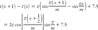
It turns out that this is true for only an integral number of miles, and that seems, frankly, rather strange. We’ll examine this case for a specific function, by redefining t(x) to be:
![]()
where m is not an integer and ε > 0. If ε is small enough and m is large enough, this will represent an increasing function with small “undulations” about the line 7.5x, representing the time to jog at the average speed. t(x) is an increasing function if t′(x) > 0, as it must be because it is a time function. Mathematically this will be so if
![]()

Figure 6.1. Lindsay’s time function t(x).
for this particular model of the jogging time. Figure 6.1 shows t(x) and the mean time function for the case ε = 1, m = 0.8.
Now it follows that
is an increasing function that can never be 7.5. Therefore if Lindsay runs so that her time function is given by equation (6.1), she will never run a complete mile in exactly 7.5 minutes.
X = T : RAINING IN THE CITY
It seems that it’s almost impossible to find a taxi when it’s raining in the city. Gene Kelly preferred to sing and dance, but, as sometimes happens when I am walking, the heavens open and I am faced with the different options of running fast or walking for shelter. Is it better to walk or run in the rain? The decision to run may seem an obvious one, but depending on several factors discussed below, it is not always that simple. And occasionally I have the foresight to take an umbrell.
What might such factors be? Among them are how fast the rain is falling, and in what direction (i.e., is there wind, and if so, in what direction), how fast I can run or walk, and how far away the shelter is. Let’s ignore the wind and rain direction initially and set up a very basic model. Suppose that you run at v m/s. Since 2 mph ≈ 1 m/s, as is easily shown, we can easily convert speeds in mph to MKS units and vice versa. Of course, this is only approximate, but we shall nevertheless use it for simplicity; we do not require precise answers here; after all, we’re in a hurry to get home and dry off!
Suppose the distance to the nearest shelter point is d km, and that the rain is falling at a rate of h cm/hr (or h/3600 cm/s). Clearly, in this simplified case it is better to run than to walk. Here is a standard classification of the rate of precipitation:
• Light rain—when the precipitation rate is < 2.5 mm (≈ 0.1 in) per hour;
• Moderate rain—when the precipitation rate is between 2.5 mm (≈ 0.1 in) and 7.6 mm (0.30 in) to 10 mm (≈ 0.4 in) per hour;
• Heavy rain—when the precipitation rate is between 10 mm (0.4 in.) and 50 millimeters (2.0 in) per hour;
• Violent rain—when the precipitation rate is > 50 mm (2.0 in) per hour.
Now if I run the whole distance d m at v m/s, the time taken to reach the shelter is d/v seconds, and in this time the amount H of rain that has fallen is given by the expression H = hd/3600v cm. If I run at 6 m/s (about 12 mph), for example, and d = 500 m, then for heavy rain (e.g., h = 2 cm/hr), H ≈ 0.5 cm. This may not seem like a lot, but remember, it is falling on and being absorbed (to some extent at least) by our clothing, unless we are wearing rain gear. The next step in the model is to estimate the human surface area; a common approach is to model ourselves as a rectangular block, but a quicker method is to consider ourselves to be a flat sheet 2 m high and 0.5 m wide. The front and back surface area is 2 m2—about right! Over the course of my run for shelter, if all that rain is absorbed, I will have collected an amount 2 × 104 × 5 × 10−2 = 103, or one liter of rain. That’s a wine bottle of rain that the sky has emptied on you! I prefer the real stuff . . .
It is important to note that rain is a “stream” of discrete droplets, not a continuous flow. It is reasonable to define a measure of rain intensity by comparing the rate at which rain is falling with the speed of the rain. The speed of raindrops depends on their size. At sea level, a very large raindrop about 5 millimeters across falls at the rate of about 9 m/s (see Chapter 25 for an unusual way to estimate the speed of raindrops). Drizzle drops (less than 0.5 mm across) fall at about 2 meters per second. We shall use 5 m/s (or 500 × 3600 = 1.8 × 106 cm/hr) as an average value. The ratio of the precipitation rate to the rain speed [13] is called the rain intensity, I. For the figures used here, I = 2/(1.8 × 106) ≈ 1.1 × 10⁻⁶. Therefore I is a parameter: I = 1 corresponds to continuous flow (at that speed), whereas I = 0 means the rain has stopped, of course!
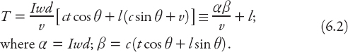
If as in Figure 6.2 the rain is falling with speed c m/s at an angle θ to the vertical direction, and you are running into it, the vertical (downward) component of speed is c cos θ and the relative speed of the horizontal component is c sin θ + v. And if you move fast enough, only the top and front of you will get wet. For now let’s assume this is the case. Since you are not in fact a thin sheet (your head does get wet), we will model your shape as a rectangular box of height l, width w and thickness t (all in m). The “top” surface area is wt m2, and the volume of rain is “collected” at a rate R = intensity × surface area × rain speed = Iwtc cos θ, expressed in units of m3/s. In time d/v the amount collected is then Iwtdc cos θ/v m3. A similar argument for the front surface area gives Iwld(c sin θ + v)/v m3, resulting in a total amount T of rain collected as
Before putting some numbers into this, note that if θ were the only variable in this expression, then
![]()
Because this vanishes at θ = arctan(l/t) and d2T/dθ2 < 0 there, this represents a maximum accumulation of rain. Physically this means that you are running almost directly into the rain, but the relative areas of your top and front are such that the maximum accumulation occurs when it is (in this case) not quite horizontal. In addition, of v were the only variable, then dT/dv = −αβ/v2 < 0 if β > 0, so that T decreases with speed v if tan θ > −t/l. If tan θ < −t/l, then T increases with speed. This corresponds to more and more negative values of θ, that is, the rain is coming from behind the runner.
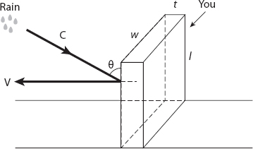
Figure 6.2. Configuration for a rectangular box-person running in the rain.
Let’s put some meat on these bones, so to speak. Suppose that the rectangular box has dimensions l = 1.5 m, w = 0.5 m, and t = 0.2 m. Furthermore, we have chosen v = 6 m/s (about 13 mph); and c = 5 m/s. Substituting all these values into expression (6.2) for T we obtain T ≈ 4.6 × 10⁻²(9 + cos θ + 7.5 sin θ) liters. It is readily confirmed that this has a maximum value of about 0.76 liters when θ ≈ 82.4°. A graph of T(θ) is shown in Figure 6.3 for −π/2 < θ < π/2. Note also that for a given speed when θ < 0 (i.e., the rain is coming from behind you) the quantity of rain accumulated is smaller (as would be expected) than when you are running into the rain. Notice also the wide range of values, from a high of just below 0.8 liters to a low of less than 0.1 liters when the rain is hitting you horizontally from behind!
We need to be a little more careful with the case of θ < 0 because (6.2) could become negative (and therefore meaningless) for some parameter ranges. If we replace θ by −![]() ,
, ![]() > 0, then this equation becomes
> 0, then this equation becomes
![]()
This is negative if
![]()
Figure 6.3. Total amount of rain captured as a function of rain angle (radians).
Note that this can never happen if v ≥ c, and will not for the choice of v and c made here (v/c = 1.2). If the inequality (6.4) is satisfied, the “offending term” comes from the “front accumulation” value
![]()
which should now be written as
![]()
because the rain falls on your back if sin v < c sin ![]() . The correct total is now
. The correct total is now
![]()
It is instructive to rewrite this equation as
![]()
Let’s focus our attention on the term in parentheses in equation (6.6), noting that t/l = Atop/Aback is just the ratio of the top area of the human “box” to the area of the back (or front). If tan ![]() > t/l = Atop/Aback, this term is negative, and in this case, you should attempt to go no faster than the horizontal speed of the rain (c sin
> t/l = Atop/Aback, this term is negative, and in this case, you should attempt to go no faster than the horizontal speed of the rain (c sin ![]() ) at your back. Using equation (6.5) we see that if your speed increases so that v = c sin
) at your back. Using equation (6.5) we see that if your speed increases so that v = c sin ![]() , you are just keeping up with the rain and T is minimized. This may seem at first surprising since for v > c sin
, you are just keeping up with the rain and T is minimized. This may seem at first surprising since for v > c sin ![]() , T is reduced still farther, but now you are catching up to the rain ahead of you, and it falls once more on your front (and head, of course). In this case formula (6.2) again applies.
, T is reduced still farther, but now you are catching up to the rain ahead of you, and it falls once more on your front (and head, of course). In this case formula (6.2) again applies.
How about putting some numbers into these formulae? For a generic height l = 175 cm (about 5 ft 9 in), shoulder to shoulder width w = 45 cm (about 18 in), and chest to back width t = 25 cm (about 10 in), the ratio t/l = 1/7, and so if tan ![]() > 1/7, that is,
> 1/7, that is, ![]() ≈ 8°, the ratio v/c = sin
≈ 8°, the ratio v/c = sin ![]() ≈ 1/7 (see why?). Therefore if it is raining heavily at about 5 m/s from this small angle to the vertical, you need only amble at less than one m/s (about 2 mph) to minimize your accumulated wetness! Although the chosen value for w was not used, we shall do so now. The top area of our human box is ≈ 1100 cm2, one side area is ≈ 4400 cm2, and the front or back area is ≈ 7900 cm2.
≈ 1/7 (see why?). Therefore if it is raining heavily at about 5 m/s from this small angle to the vertical, you need only amble at less than one m/s (about 2 mph) to minimize your accumulated wetness! Although the chosen value for w was not used, we shall do so now. The top area of our human box is ≈ 1100 cm2, one side area is ≈ 4400 cm2, and the front or back area is ≈ 7900 cm2.
Exercise: Calculate these areas in square feet if you feel so inclined.
To summarize our results, if the rain is driving into you from the front, run as fast as you safely can. On the other hand, if the rain is coming from behind you, and you can keep pace with its horizontal speed by walking, do so! If you exceed that speed, the advantage of getting to your destination more quickly is outweighed by the extra rain that hits you from the front, since you are now running into it! Perhaps the moral of this is that we should always run such that the rain is coming from behind us!
X = ΔT: WEATHER IN THE CITY
To some extent cities can create their own weather. No doubt you have heard of the sidewalk in some city being hot enough to fry an egg; include all the paved surfaces and buildings in a city, and you have the capacity to cook a lot of breakfasts! Typically, such surfaces get hotter than those in rural environments because they absorb more solar heat (and therefore reflect less), and retain that heat for longer than their rural counterparts by virtue of their greater thermal “capacity.” The contrast between a city and the surrounding countryside is further enhanced at night, because the latter loses more heat by evaporative and other processes. Furthermore, the combined effects of traffic and industrial plants are a considerable source of heat within an urban metropolitan area. Thus there are several factors to take into account when considering local climate in a city versus that in the countryside. They include the fact that (i) there are differences between surface materials in the city and the countryside—concrete, tarmac, soil, and vegetation; (ii) the city “landscape”—roofs, walls, sidewalks, and roads—is much more varied than that in the country in the shape and orientation of reflective surfaces; vertical walls tend to reflect solar radiation downward instead of skyward (see Figure 6.4a,b), and concrete retains heat longer than do soil and vegetation; (iii) cities are superb generators of heat, particularly in the winter months; (iv) cities dispose of precipitation in very different ways, via drains, sewers, and snowplows (in the north). In the country, water and snow are more readily available for evaporative cooling.
Such local climate enhancement has several consequences, some of which are positive (or at least appear to be). For example, there may be a diminution of snowfall and reduced winter season in the city. This induces an earlier spring, other species of birds and insects may take up residence, and longer-lasting higher temperature heat waves can occur in summer (quite apart from any effects of larger scale climate change). This in turn means that less domestic heating may be required in the winter months, but more air-conditioning in the summer. The effects of an urban-industrial complex on weather generally are harder to quantify, though stronger convective updrafts (and hence intensity of precipitation and storms) are to be expected downwind from urban areas. According to one report (Atkinson 1968), there has been a steadily increasing frequency of thunderstorm activity near London as it has grown in size. In U.S. cities, the incidence of thunderstorms is 10–42% greater than in rural areas, rainfall is 9–27% greater and hailstorms occur more frequently, by an enormous range: 67–430%.
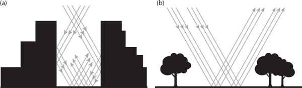
Figure 6.4. (a) Vertical surfaces tend to reflect solar radiation toward the ground and other vertical surfaces (thus trapping it), especially when the sun’s elevation is moderately high. (b) There being fewer vertical surfaces in the countryside, solar radiation tends to be reflected skyward. Redrawn from Lowry (1967).
If the air temperature were to be recorded as we move across the countryside toward a city, the rural/urban boundary will typically exhibit a sharp rise—a “cliff”—followed by a slower rate of increase (or even a plateau) until a more pronounced “peak” appears over the city center. If the temperature difference between the city and surrounding countryside at any given time is denoted by ΔT, the average annual value for ΔT ranges from 0.6 to 1.8°C. Of course, the detailed temperature profile as a function of position will vary depending on the time of day, but generally this is a typical shape: a warm “island” surrounded by a cooler “sea.” Obviously the presence of parks and other open areas, lakes, and commercial, industrial and heavily populated areas will modify this profile on a smaller spatial scale. The difference ΔT between the maximum urban temperature and the background rural temperature is called the urban heat island intensity. Not surprisingly, this exhibits a diurnal variation; it is at a maximum a few hours after sunset, and a minimum around the middle of the day. In some cases at midday the city is cooler than its environs, that is, ΔT < 0.
To see why this might be so, note that near midday the sunlight strikes both country and city environs quite directly, so ΔT can be small, even negative, possibly because of the slight cooling effect of shadows cast by tall buildings, even with the sun high overhead. As the day wears on and the sun gets lower, the solar radiation strikes the countryside at progressively lower angles, and much is accordingly reflected. However, even though the shadows cast by tall buildings in the city are longer than at midday, the sides facing the sun obviously intercept sunlight quite directly, contributing to an increase in temperature, just as in the hours well before noon, and ΔT increases once more.
Cities contribute to the “roughness” of the urban landscape, not unlike the effect of woods and rocky terrain in rural areas. Tall buildings provide considerable “drag” on the air flowing over and around them, and consequently tend to reduce the average wind speed compared with rural areas, though they create more turbulence (see Chapter 3). It has been found that for light winds, wind speeds are greater in inner-city regions than outside, but this effect is reversed when the winds are strong. A further effect is that after sunset, when ΔT is largest, “country breezes”—inflows of cool air toward the higher temperature regions—are produced. Unfortunately, such breezes transport pollutants into the city center, and this is especially problematical during periods of smog.
Question: Why is ΔT largest following sunset?
This is because of the difference between the rural and urban cooling rates. The countryside cools faster than the city during this period, at least for a few hours, and then the rates tend to be about the same, and ΔT is approximately constant until after sunrise, when it decreases even more as the rural area heats up faster than the city. Again, however, this behavior is affected by changes in the prevailing weather: wind speed, cloud cover, rainfall, and so on. ΔT is greatest for weak winds and cloudless skies; clouds, for example, tend to reduce losses by radiation. If there is no cloud cover, one study found that near sunset ΔT ∝ w−1/2, where w is the regional wind speed at a height of ten meters (see equation (6.7)).
Question: Does ΔT depend on the population size?
This has a short answer: yes. For a population N, in the study mentioned above (including the effect of wind speed), it was found that
![]()
though other studies suggest that the data are best described by a logarithmic dependence of ΔT on log10 N. While every equation (even an approximate one) tells a story, equation (6.7) doesn’t tell us much! ΔT is weakly dependent on the size of the population; according to this expression, for a given wind speed w a population increase by a factor of sixteen will only double ΔT! And if there is no wind? Clearly, the equation is not valid in this case; it is an empirical result based on the available data and valid only for ranges of N and w.
Exercise: “Play” with suitably modified graphs of N1/4 and log10 N to see why data might be reasonably well fitted by either graph.
The reader will have noted that there is not much mathematics thus far in this subsection. As one might imagine, the scientific papers on this topic are heavily data-driven. While this is not in the least surprising, one consequence is that it is not always a simple task to extract a straightforward underlying mathematical model for the subject. However, for the reader who wishes to read a mathematically more sophisticated model of convection effects associated with urban heat islands, the paper by Olfe and Lee (1971) is well worth examining. Indeed, the interested reader is encouraged to consult the other articles listed in the references for some of the background to the research in this field.
To give just a “taste” of the paper by Olfe and Lee, one of the governing equations will be pulled out of the air, so to speak. Generally, I don’t like to do this, because everyone has the right to see where the equations come from, but in this case the derivation would take us too far afield. The model is two-dimensional (that is, there is no y-dependence), with x and z being the horizontal and vertical axes; the dependent variable θ is essentially the quantity ΔT above, assumed to be small enough to neglect its square and higher powers. The parameter γ depends on several constants including gravity and air flow speed, and is related to the Reynolds number discussed in Chapter 3. The non-dimensional equation for θ(x, z) is
![]()
The basic method is to seek elementary solutions of the form
![]()
where “Re” means that the real part of the complex function is taken, and k is a real quantity On substituting this into equation (6.8) the following complex biquadratic polynomial is obtained:
![]()
There are four solutions to this equation, namely,
![]()
but for physical reasons we require only those solutions that tend to zero as z → ∞. The two satisfying this condition are those for which Re σ < 0,
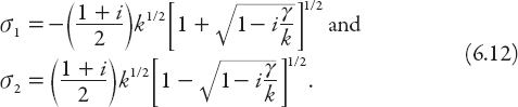
Using these roots, the temperature solution (6.9) can be expressed in terms of (complex) constants c1 and c2 as
![]()
Note from equation (6.12) that ![]() Using specified boundary conditions, both c1 and c2 can be expressed entirely in terms of σ1 and σ2, though we shall do not do so here. The authors note typical magnitudes for the parameters describing the heat island of a large city (based on data for New York City). The diameter of the heat island is about 20 km, with a surface value for ΔT ≈ 2C, and a mean wind speed of 3 m/s.
Using specified boundary conditions, both c1 and c2 can be expressed entirely in terms of σ1 and σ2, though we shall do not do so here. The authors note typical magnitudes for the parameters describing the heat island of a large city (based on data for New York City). The diameter of the heat island is about 20 km, with a surface value for ΔT ≈ 2C, and a mean wind speed of 3 m/s.