Chapter 12

CAR FOLLOWING IN THE CITY—II

I love to watch clouds; their changing forms are indicative of the different kinds of hydrodynamical process that are present in the upper atmosphere, such as convection, shear flow, and turbulence. Unfortunately, I am rather prone to do this while driving. Probably the worst example of this occurred many years ago when my wife and I were on our way to the local hospital (she was in labor with our third child). I won’t elaborate here, except to say that she rightly urged me to concentrate on the road. Distractions such as cloud-watching while driving increase the reaction time for avoiding traffic hazards (and therefore should not be engaged in!). This next set of models incorporate reaction times in a simple and rather natural manner.

X = Q: ALTERNATIVE CAR-FOLLOWING MODELS

We now consider a driver traveling at speed u who tries to maintain a constant distance between his car and the one ahead of him. Since he will wish to be able to stop suddenly if the vehicle ahead does, and to do so without hitting it, the spacing s can be written (in particular) as a quadratic function of speed. (Why is this so?) Consider the expression

From equation (12.1) the constants s₀, a, and b must have dimensions of distance, time, and (acceleration)⁻¹, respectively. Therefore s₀ might be, for instance, the minimum spacing from the back of car n to the front of the following car (n − 1) or front to front. The constant a could be the reaction time to a sudden braking of the car ahead, and b could be the maximum deceleration, which would modify the speed u in order to keep s constant. We can solve equation (12.1) for u:

where α = a/s₀ and β = b/s₀. The positive solution (+ root) can be recast directly into a form related to q = q(k) by defining some new parameters:

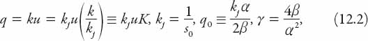
from which we obtain the expression

In view of the above discussion about the shape of the q(k) (and now the q(K)) graph, we seek the location of the maximum from dq/dK = 0, that is, where

Simplifying, we obtain the following quadratic equation in K:

This equation has the roots

On substituting these into equation (12.3) it transpires that only the – root gives q > 0. We can write this value as

Finally, writing Q = q/q_max we have an expression for Q(K), that is,

A typical graph of Q(K) is shown in Figure 12.1. The maximum occurs at

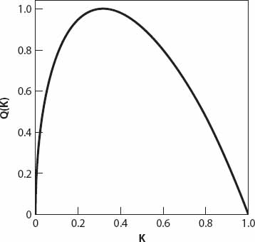
Figure 12.1. Modified q-k diagram based on equation (12.6).

The position of the maximum changes relatively little with γ; in the interval 1 < γ < ∞, for example, 0.25 < K_m < 0.5.

Note also that

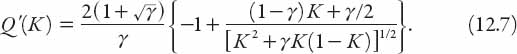
This explains the shape of the graph near the origin; as K → 0⁺, Q′(K) → ∞ (as does q′(k) of course). As the concentration goes to zero, any interaction between vehicles will become negligible, and the flow would become an average “free speed,” which renders this car-following model inapplicable. In practice, the real flow at any concentration is probably less than this, so the slope of the graph near the origin will not be so steep (see Figure 10.1).

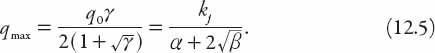
In closing this section, let us revisit equation (12.5) for the capacity q_max. In terms of the original parameters (see equation (12.1))

It is clear from this formula that the capacity can be raised by decreasing the reaction time (a), decreasing the headway distance (s₀), or increasing the desired maximum deceleration (b⁻¹) (not a good idea), or indeed, any combination of these changes. Conversely, the capacity will be lowered by changing them in the opposite directions.

It is appropriate to mention an “equation” from the field of psychology in this context, namely “Response = Sensitivity × Stimulus.” The response is usually identified as the acceleration (or deceleration) of the following vehicle, and experimental studies have shown that there is a high correlation between a driver’s response and the relative speed of the vehicle ahead—the stimulus. With this in mind, note that differentiation of equation (12.1) with respect to t yields

This is a type of stimulus-response equation, although the sensitivity term (a + 2bu)⁻¹ decreases with increasing speed u, so it is not a particularly useful interpretation in this regard.

X = u_n: AN IMPROVED REACTION-TIME MODEL

There is another avenue worth pursuing in connection with the reaction time T. If we define s_n = x_n−1 − x_n as the spacing ahead of the nth car (at location x_n), rewrite equation (11.3) in terms of the discrete speed u_n = dx_n/dt, and let t → t − T, this equation becomes (with c_n = 0)

This differential-difference can be solved exactly using more advanced techniques, but we will use an approximate method consistent with the level of this book. We can expand the right-hand side of this equation as a Taylor series about t; retaining up to the quadratic term in T we obtain the expression

Now

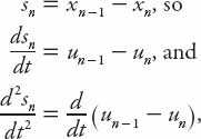
and so on. Placing all the terms involving u_n on the left-hand side, and all those in u_n−1 on the right, we have the following constant coefficient second-order nonhomogeneous ordinary differential equation (quite a mouthful):

If we know the speed of vehicle (n − 1), this equation enables us in principle to find the speed of the following vehicle (n). From the elementary theory of differential equations we know that the general solution of this equation is the sum of the solution to the homogeneous equation (i.e., with zero right-hand side) and a particular solution to the complete equation (with the right-hand side being a known function of t). The former solution is the most important determinant of the instability of the traffic flow, so we seek solutions of equation (12.10) in the form u_n(t) = Ue^pt, where U is a constant. There are two values of the constant p to be found by substitution. These values are roots of the quadratic equation

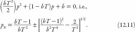
The nature of p (and hence the solution) depends on the sign of the radicand; it will be real (and hence non-oscillatory), provided

Otherwise the roots are complex conjugates, and the sign of the real part determines the solution behavior. If

(i) 0 ≤ bT ≤ − 1; both roots are negative and the solution is exponentially decreasing (stable).

 (ii) − 1 < bT < 1; both roots are complex, and the solution is damped oscillatory (stable).

(iii) bT = 1; both roots are pure imaginary, and the solution is oscillatory (neutrally stable).

(iv) bT > 1; both roots are complex, and the solution is increasing and oscillatory (unstable).

What does all this mean? Remember that the solution u_n(t) = Ue^pt is the speed of the nth vehicle in the line of traffic. From cases (i)–(iv) we see that (locally at least) the speed can decrease, oscillate about a decreasing mean value, oscillate about a constant mean value, and oscillate about an increasing mean value. This last case is indicative of the potential for collisions somewhere down the traffic line. The model is a crude one, to be sure, but this latter behavior is also consistent with the solution for the nonhomogeneous equation, known as the “particular integral.” The choice of functional form sought depends on that of the presumed known quantity u_n−1(t), but for our purposes it is sufficient, in light of (i)–(iv) above to consider an oscillatory solution of the form . Substituting this in equation (12.10) results in the expression

Note that

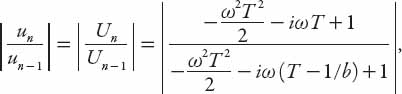
and this ratio grows as n increases if the expression on the right exceeds unity. Note that this term can be written in simplified form in terms of real and imaginary parts as

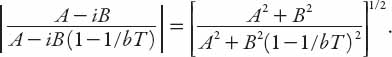
It is clear that we require bT > 1/2 for |u_n/u_n−1| > 1. This then supersedes the previous criterion for instability because it “kicks in” at a lower value of bT.

For completeness in this section, the exact solution for this problem is stated below:

(i) 0 ≤ bT ≤ e⁻¹ ≈ 0.368; both roots are negative and the solution is exponentially decreasing (stable).

 (ii) e⁻¹ < bT < π/2 ≈ 1.571; both roots are complex, and the solution is damped oscillatory (stable).

(iii) bT = π/2; both roots are pure imaginary, and the solution is oscillatory (neutrally stable).

(iii) bT > π/2; both roots are complex, and the solution is increasing and oscillatory (unstable).

The rough and ready calculations therefore have the right “character traits” insofar as stability and instability are concerned, but the transition points are inaccurate. However, it must be said that compared with the exact solution, the upper bound in part (i) above is an overestimate of only 11%, while the transition value in part (iii) is an underestimate of about 36%.

Exercise: Show that, had we expanded equation (12.9) as a linear Taylor polynomial in T only, the results would have been very similar:

for the homogeneous solution and