Chapter 14

ROADS IN THE CITY

X = : Question: What is the average distance traveled in a city/town center?

This can be quite a complicated quantity to calculate, depending as it does on the type of road network and distribution of starting points and destinations, among other factors. Smeed (1968) assumed a uniform distribution of origins and destinations for both idealized and real UK road networks, and with some simplifying assumptions, concluded that the range of values lay between 0.70A^1/2 and 1.07A^1/2, with a mean of 0.87A^1/2, A being the area of the town center (assuming this can be suitably defined). Obviously the factor A^1/2 renders the result dimensionally correct. With this behind us, the next stage is to try to determine the average length of a journey during say, a peak travel period. Using rather sophisticated statistical tools, Smeed was able to calculate the above average distance traveled on roads of any given town or city center, assuming only that the journeys are made by the shortest possible route. Rather than try to reproduce the (unpublished) calculations here, let us try to make these figures plausible on the basis of some simple geometric models of cities.

We will just calculate the mean lengths of parallel roads in circular and rectangular town centers as we move from one side of the town center to the other. Even this rather crude approach yields answers close to those found in the literature, indicating that the coefficient is relatively insensitive to the structure of the road network. First, we consider a set of N-S parallel roads in a circular town center of radius r (see Figure 14.1), separated by a constant distance r/n, where n is a positive integer. In so doing, we are neglecting the combined width of the road network compared with the town center area. Each road passing within a distance pr/n of the origin (where p is an integer less than n) has length 2r[1 − (p/n)²]^1/2, and for each p > 0 there are two roads of identical length. There are 2(n − 1) + 1 = 2n − 1 roads, so the discrete average length is given by

Of course, an identical result holds for W-E roads, and the combined average will be the same. To express in terms of A^1/2 we merely write = kA^1/2 = kπ^1/2r, so that the coefficient . For n = 3 (five roads), k ≈ 0.99; for n = 4 (seven roads), k ≈ 0.96, and for n = 10 (nineteen roads), k ≈ 0.92. Thus we see that these constants are well within the range found by Smeed.

Figure 14.1. Cartesian road “grids” in rectangular (shown here, square) and circular cities.

It may be of some interest to take the mathematical limit as n → ∞, in the above equation and calculate the average length for a continuum of roads—perhaps more appropriate for ducks on a circular pond (though possibly a good description of the morning commute!). In practice, it is less messy just to set up the integral for the average value of the function L(x) = 2(r² − x²)^1/2, that is,

This is a standard integral, and can be evaluated with a trigonometric substitution to find that

Hence, proceeding as before, setting πr/2 = kA^1/2 yields . It would appear that this is indeed the limit of the decreasing sequence of k-values suggested by equation (14.1).

Exercise: (a) Verify this result for ; (b) find k for n = 100.

Now we proceed to evaluate and k for a rectangular town center. We suppose that the longer sides are parallel to the x-direction, for convenience. The sides are of length a, and b > a. There are n + 1 N-S equally spaced roads (including the sides) and, similarly, m + 1 W-E equally spaced roads. We assume the N-S and W-E road spacing is the same, Δ, say. The average distance traveled (again, from side to opposite side, for simplicity) is

If we let b = (1 + α)a, this can be rearranged to give

The parameter α is a measure of how “rectangular” the town center is; the smaller the value of α the closer the center is to being square. Furthermore, since we wish to write and A = ab = (1 + α)a², it follows that

This can be simplified still further by noting that, since a = mΔ and b = nΔ,

Substituting for n we find that, after a little rearrangement,

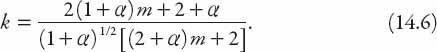
Figure 14.2 shows excellent agreement for bounds on k(α) when compared with the range quoted by Smeed. In passing, it is worthwhile to note that the topics discussed here are related to the probabilistic one of determining the average distance between two random points in a circle. A simple derivation of one such result can be found in Appendix 7. There has been much in the mathematical literature devoted to this problem, and it has been adapted by several theoretical urban planning groups to model optimal traffic routes between centers of interest.

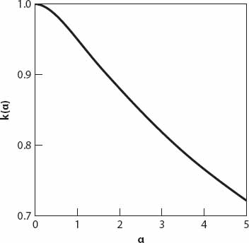
Figure 14.2. Proportionality parameter k (see equation (14.5)) as a function of α (m = 10 here).

X = T_i: Question: What difference does a beltway make?

A beltway (or ring road in the UK) is a highway that encircles an urban area so that traffic does not necessarily have to pass through the center. A driver wishing to get to the other side of the city without going through the center might be well advised to use this alternative route. However, I’ve heard it said regarding the M25 motorway (a beltway around outer London) that it can be the largest parking lot in the world at times! Nevertheless, in my (somewhat limited) experience, a combination of variable speed limits and traffic cameras usually keeps the traffic flowing quite efficiently via a feedback mechanism between the two.

As always in our simple models, circular cities will be considered to be radially symmetric; that is, properties vary only with distance r. The city is of radius r₀ and v(r) is the speed of traffic (in mph) at a distance r from the city center, 0 ≤ r ≤ r₀. V₀ is the speed of traffic around the (outer) beltway from any starting point A on the perimeter. For simplicity we will assume that V₀ is constant and that v(r) is a linearly increasing function; as we will see, even these simplistic assumptions are sufficient to provide some insight into the potential advantages of a beltway. Thus v(r) = ar + b, a ≥ 0, b ≥ 0. A driver wishes to travel from point A to point P(r₀, θ), (see Figure 14.3) both situated on the perimeter road. We shall suppose that there is also a circular “inner city” beltway a distance r₁ < r₀ from the center O, along which the constant speed is V₁ ≤ V₀. She then has three choices: (1) to drive right into the city center and out again to P, the path ADOFP; (2) to drive around the outer beltway along path ABP, and (3) to take an intermediate route using the inner beltway along the path ADEFP. We shall calculate the times taken along each route under our stated assumptions.

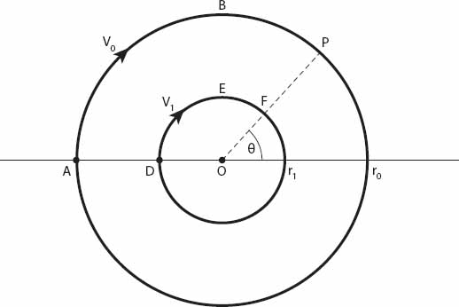
Figure 14.3. Radially symmetric velocity contours in a circular city.

For the first choice, noting that v = dr/dt, we have that

For the second route,

Finally, for the third route, involving some travel around the inner beltway,

Obviously this last case is intermediate between the other two in the sense that as the inner beltway radius r₁ → 0, T₃ → T₁, and as the outer radius r₁ → r₀, T₃ → T₂. It is interesting to compare these travel times; so let us examine the first two cases and ask when it is quicker to travel along the outer beltway to P, that is, when is T₂ < T₁? This inequality can be arranged as

Since f₁(0) = f₂(0) = 0, and , it follows that the graphs of these two functions will intersect at some radius, r_c say, if and only if , i.e., if 2V₀ > (π − θ)b. If r_c < r₀ then there will be an interval (0, r_c) for which it is quicker (in this model) to travel along the outer beltway to P. If r_c > r₀ then the curves do not intersect and it is always quicker to use the outer beltway.